Highlighting with conditional formating

[jbrown021286]

I am building a spreadsheet that is going to be used as a double check for paid accounts. In colum A I will have several accounts and in colum D I am wanting to past a list of accounts that are paid. Is there a way to use conditional formating to highlight any cell in colum A and any cell in colum D that has a matching number in the opsing colum?

 

[Joe4]

So, for row 2, you would select cells A2 and D2 and you would set up a Conditional Formatting Rule formula like:

=$A2=$D2

and choose your formatting option.

 

[jbrown021286]

So, for row 2, you would select cells A2 and D2 and you would set up a Conditional Formatting Rule formula like:

=$A2=$D2

and choose your formatting option.

The matching numbers would most likly not be in the same row so that wouldn't work past the first fee rows once a number was skipped because it wasn't in the list of colum D

 

[Joe4]

The matching numbers would most likly not be in the same row so that wouldn't work past the first fee rows once a number was skipped because it wasn't in the list of colum D

OK, that is not very clear from your original description.
Can you please post a small sampling of what your data actually looks like and your expected results?

MrExcel has a tool called “XL2BB” that lets you post samples of your data that will allow us to copy/paste it to our Excel spreadsheets, so we can work with the same copy of data that you are. Instructions on using this tool can be found here: XL2BB Add-in

Note that there is also a "Test Here” forum on this board. This is a place where you can test using this tool (or any other posting techniques that you want to test) before trying to use those tools in your actual posts.

My best guess without seeing your data is I am thinking then you may need two rules.
For the first one, select column A, then enter this Conditional Formatting formula:

=COUNTIF(D:D,A1)>0

and choose your desired formatting option.

And then do something similar for the second, selecting column D, and using this Conditional Formatting formula:

=COUNTIF(A:A,D1)>0

and choose your desired formatting option.

 

[jbrown021286]

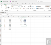
this is a very basic example of the account spreadsheet, as you can see in column A and D i have account numbers and in Colum b I have invoice amount and column e I have how much has been paid to the balance of the account. i am wanting to be able to highlight all the accounts that are matched from both column a and d as well as highlight the balance if the balance matches in column b and e. is this possible?

 

[Joe4]

Did you try what I suggested in my previous post? That would do what you want for columns A and D.

To do all four columns, follow these rules. I used different formatting colors so you could see where each is coming from.

Rule 1:
Select column A
Use Conditional Formatting formula:

=COUNTIF(D:D,A1)>0

Choose highlighting color yellow.

Rule 2:
Select column D
Use Conditional Formatting formula:

=COUNTIF(A:A,D1)>0

Choose highlighting color green.

Rule 3:
Select column B
Use Conditional Formatting formula:

=COUNTIFS(D:D,A1,E:E,B1)>0

Choose highlighting color blue.

Rule 4:
Select column E
Use Conditional Formatting formula:

=COUNTIFS(A:A,D1,B:B,E1)>0

Choose highlighting color orange.

So, in the end, it looks like this:

 

[jbrown021286]

Did you try what I suggested in my previous post? That would do what you want for columns A and D.

To do all four columns, follow these rules. I used different formatting colors so you could see where each is coming from.

Rule 1:
Select column A
Use Conditional Formatting formula:

=COUNTIF(D:D,A1)>0

Choose highlighting color yellow.

Rule 2:
Select column D
Use Conditional Formatting formula:

=COUNTIF(A:A,D1)>0

Choose highlighting color green.

Rule 3:
Select column B
Use Conditional Formatting formula:

=COUNTIFS(D:D,A1,E:E,B1)>0

Choose highlighting color blue.

Rule 4:
Select column E
Use Conditional Formatting formula:

=COUNTIFS(A:A,D1,B:B,E1)>0

Choose highlighting color orange.

So, in the end, it looks like this:
View attachment 87576

that worked great this is the spreadsheet that I built around that. the column named RO is column A in my previous example, Flag Time would be B, RO Check would be C and Hours check would be D. is there a good way of calculating the column "adjustment" in with the flag time so that if the sum of the 2 is equal to the corresponding hours check it would highlight it as well?

 

[Joe4]

is there a good way of calculating the column "adjustment" in with the flag time so that if the sum of the 2 is equal to the corresponding hours check it would highlight it as well?

That appears to be a vastly different question that your original question.
As such, you should post it to a brand new thread. Then it will show up as a new unanswered question in the "Unanswered threads" listing, and have a much better chance of being seen and answered.

 

[jbrown021286]

That appears to be a vastly different question that your original question.
As such, you should post it to a brand new thread. Then it will show up as a new unanswered question in the "Unanswered threads" listing, and have a much better chance of being seen and answered.

Ok. Thanks for all your help