Horizontal indexing from large array

[Hordern]

Hi Folks

I've only been getting to grips with tougher formulae in the last 36 hours and I've achieved most things that I wish to - partly thanks to some wonderful explanations in these forums. However, I'm struggling on the last step and I can't find a thread that answers it.

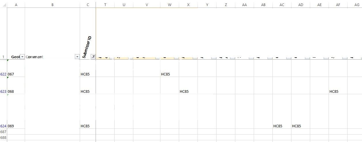
I have an array that is over 600 rows deep and around 30 columns across. Column A is an location ID number, B is irrelevant to this query. C contains a submitter ID number and D is also irrelevant. Every column after that is a feature of the location and where a submitter has commented on that feature at that location, I have included their submitter number.

I have multiple rows with the same locations, and multiple rows with the same submitter, but never a repeat of a location and submitter.


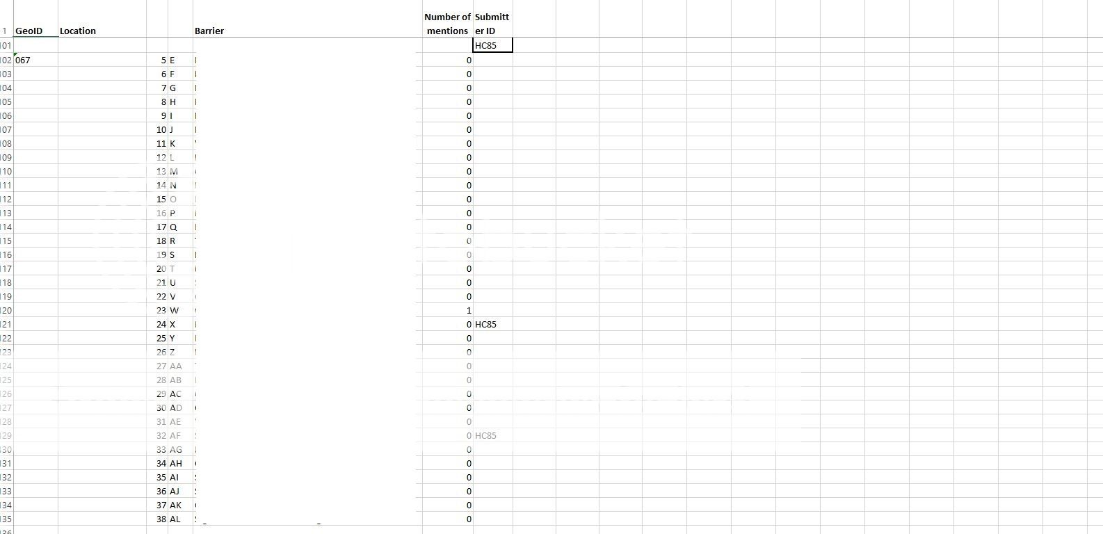
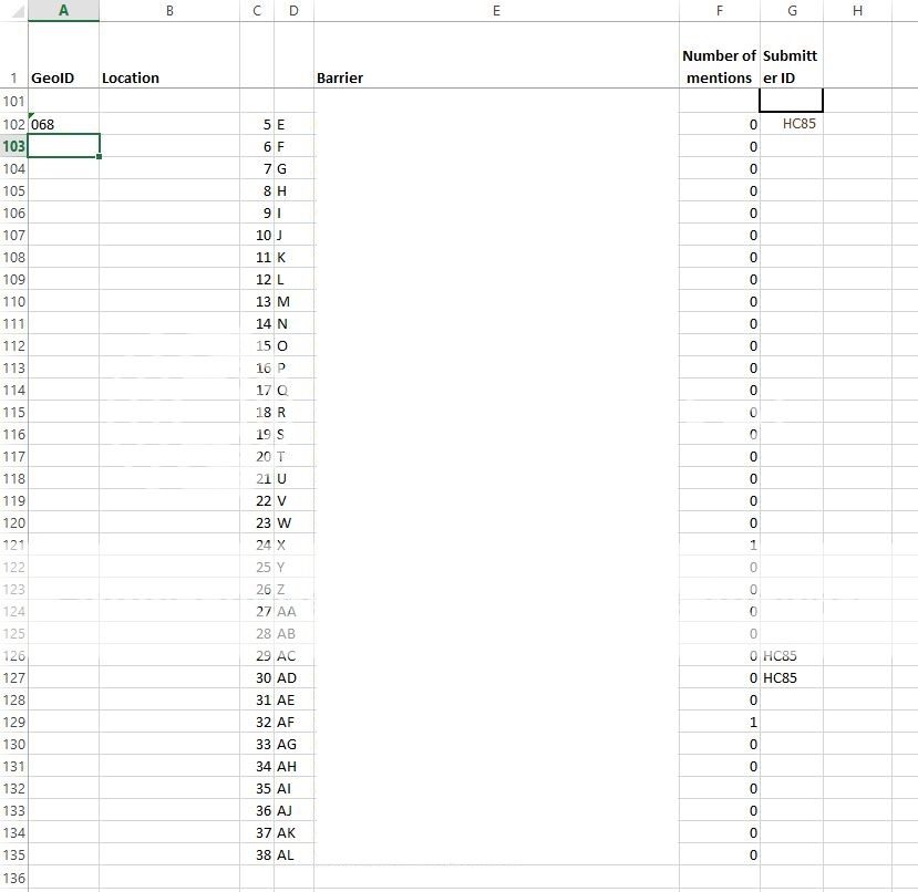
On another page I am listing the location ID in A. B is irrelevant to this, C has the column headers from the array (these will be copied again and again as necessary) and D has the number of submitters who have commented about the feature in the location (I used this: =COUNTIF(BarriersGeo!E:E,A102) where BarrieraGeo is the tab name, E:E is the feature column and A102 is the location ID within the indexing tab).

Now in E I am trying to list the submitters who have contributed to that location and feature.

I managed to get it to work where there was only 1 submitter for a given location ID by using:

=VLOOKUP(A102,BarriersSub!A2:AL686,17,0)

Where 17 is a feature column.


After playing with google and some tutorials I got as far as the following with CSE to make it an array:

=INDEX(BarriersSub!$E$2:$E$686, SMALL(IF($A$102=BarriersSub!$A$2:$A$686, ROW(BarriersSub!$A$2:$A$686)-ROW(BarriersSub!$A$2)+1), ROW(1:1)))

When I drag this down the column, I get a cell for every time the location ID is listed in the array table. The cell is blank if the submitter did not choose the feature being indexed and the submitter number. The cell has the submitter number if the submitter commented on that feature.

The MAIN thing I'd like to fix is being able to drag the formula horizontally (I tried playing with ROW and COLUMN but got nowhere). Preferably with an IF in the correct place to ignore the blank references [I'm 99% sure this can be done]. Ideally I'd like all the submitters to be listed in one cell but that doesn't really matter very much and I'm not expecting that to be possible.

My mind is melting right now as up until 2 days ago the most I'd done was use SUM and TOTAL...

I hope this makes sense and thank you so much in advance.

 

[Hordern]

Wow, Posted on Friday afternoon, it's now Monday morning and it's already on page 22!

If it would be helpful for me to post some sample data, please let me know. If I find some time today (I have to access from work as home internet is too unreliable/slow) I'll get an example up.

 

[FDibbins]

See if this will get you started. In the sample below, I have created the INDEX/SMALL both ways, using the same data...

	A​	B​	C​	D​	E​	F​	G​	H​	I​
1​	Headre1	Header2	headre3	Header4		10​
2​	10​	cat	cat 123	cat456		cat​	cat 123	cat 123	cat 126
3​	10​	dog	dog 124	dog456			cat 126
4​	20​	fish	fish 125	fish456
5​	10​	cat	cat 126	cat456
6​	30​	dog	dog 127	dog456
7​	30​	fish	fish 128	fish456
8​	40​	cat	cat 129	cat456
9​	40​	dog	dog 130	dog456
10​	50​	fish	fish 131	fish456

F1 and F2 are the search criteria
G2=IFERROR(INDEX(C:C,SMALL(IF(($A$2:$A$10=$F$1)*($B$2:$B$10=$F$2),ROW($A$2:$A$10)),ROWS($A$1:A1))),"")
ARRAY formula, copied down

OR...
H2=IFERROR(INDEX($C:$C,SMALL(IF(($A$2:$A$10=$F$1)*($B$2:$B$10=$F$2),ROW($A$2:$A$10)),COLUMNS($A$1:A1))),"")
ARRAY entered, copied across

 

[Hordern]

Thank you SO much Ford

Massive thumbs up and I'd give you a hug if I knew you better and thought you might appreciate it! You have what is probably your pet dog as your avatar so you probably would

 

[FDibbins]

Hugs are always good, so thanks - and yes, that was my old dog, she made it to 16

Glad to help

 

[Hordern]

Hmmm, pity we can't edit.

Something odd has happened, it seems to get out of synch with itself after a few reference changes. I need to get this spreadsheet done for now, so will combine what I had before with some of the above info to do it semi-manually for now and will then explain what's going on in more detail and with some of my own data to make things clearer when I have time.

 

[FDibbins]

Are you entering using CTRL SHIFT ENTER, and not just enter?

based on my formula...
H2=IFERROR(INDEX($C:$C,SMALL(IF(($A$2:$A$10=$F$1)*($B$2:$B$10=$F$2),ROW($A$2:$A$10)),COLUMNS($A$1:A1))),"")

INDEX($C:$C
This is pulling data from C, if you are starting in a different column, adjust as needed

($A$2:$A$10=$F$1)*($B$2:$B$10=$F$2)
These are the ranges that your criteria are in, again, adjust as needed, but make sure they match

ROW($A$2:$A$10))
This range also needs to match the criteria ranges

COLUMNS($A$1:A1)
This needs to stay as-is

 

[Hordern]

OK, so I've discovered one issue so I've taken a couple of screenshots which hopefully shows what's happening:

This is the tab called BarriersSub. It has been filtered by SubmitterID in Column C. Column B is just the comments that the rest of the table is derived from. Row 1 is a list of the various barriers encountered in the study. As you can see, I have multiple comments from individual submitters as they correspond to different locations or GeoID's. However, multiple submitters will mentioned the same GeoID, so there are multiple instances of many of the GeoID's in Column A, and multiple instances of various Submitter ID's in Column C. There should however be no repetition of the same combination (I entered all the info manually so I know this to be the case).

The next image shows the tab in which I'm trying to index this stuff. Column E lists the barriers in the same order that they are listed in Row 1 in the previous tab (Column D shows the column reference from the previous tab to make it easier for me to check, and Column C is the column 'number' for my VLOOKUP in cell G101).

Column F shows the number of times the particular barrier is mentioned for the given GeoID. In cell F for instance I use the formula: =COUNTIF(BarriersGeo!E:E,$A$102). this column is working as intended

I used the following array formula in G102: =IFERROR(INDEX(BarriersSub!$E$2:$E$686,SMALL(IF($A$102=BarriersSub!$A$2:$A$686,ROW(BarriersSub!$A$2:$A$686)),COLUMNS($A$1:A1))),"").

The formula copies down the column except I change the $E$2:$E$686 to the matching letter reference in the row as shown in column D. I then drag all of the array formulas across in one go.

As you can see, this shows 2 instances of submitter HC85 mentioning barriers at the GeoID 067 - barriers X and AF. However, the counter in column F only shows 1 mention of a barrier at this location, and it's a different barrier [W]. As you can see from the first image, HC85 does indeed mentioned barrier W at GeoID 067. However, the array formula has chosen to show the barriers mentioned by the same submitter at a different GeoID [068].

Can anyone see where I've gone wrong?

Many thanks.

 

[Hordern]

Interestingly, when I type in the next GeoID [068], the array formula displays the HC85 in the positions for GeoID 069 and you can see the counters in Column F are showing the correct info for GeoID 068

 

[FDibbins]

OK I see 1 error there...
=IFERROR(INDEX(BarriersSub!$E$2:$E$686,SMALL(IF($A$102=BarriersSub!$A$2:$A$686,ROW(BarriersSub!$A$2:$A$686)),COLUMNS($A$ 1:A1))),"")

If you notice, in my suggested formula, I used the entire column there E:E, not a range.

Try that and see if that fixes it

Also, I thought you had 2 criteria to test against? Your formuyla just shows 2
H2=IFERROR(INDEX($C:$C,SMALL(IF(($A$2:$A$10=$F$1)*($B$2:$B$10=$F$2),ROW($A$2:$A$10)),COLUMNS($A$1:A1))),"")