Hello,
I am somewhat of a novice to excel/gsheet and really need some help.
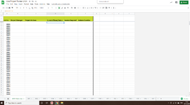
Currently creating a '2021 job tracker' and need the 'Overview' page to sync to certain cells in each individual job tracker.
See attached.
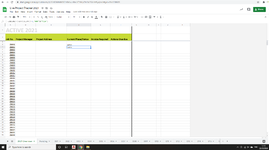
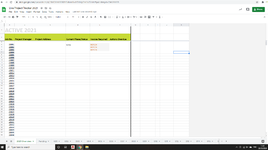
Cell D3 =MASTER!C24
I then need Cell D4 to say =001!C24, Cell D5 to say =002!C24, Cell D6 to say =003!C24... then 004, 005, 006 and so on.
Is there a way to do this automatically without having to update each individual formula?
Thank you in advance!!")
I am somewhat of a novice to excel/gsheet and really need some help.
Currently creating a '2021 job tracker' and need the 'Overview' page to sync to certain cells in each individual job tracker.
See attached.
Cell D3 =MASTER!C24
I then need Cell D4 to say =001!C24, Cell D5 to say =002!C24, Cell D6 to say =003!C24... then 004, 005, 006 and so on.
Is there a way to do this automatically without having to update each individual formula?
Thank you in advance!!