Greetings,
I have sales numbers for each Distributor. we have a new policy that Distributors will get free units from the mother company if they meet the target. But the problem is this free unit should be calculated based on cumulative sales and counted from the maximum target. Thus, seeking the expert help, please.
An example is given below:
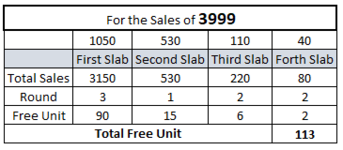
Assume that the distributor sales 3999 unit in a month. thus, free unit calculation is
=1050*3=3150 which will be equivalent to 30*3
Rest, 849, which will be under 530 sales quantity. And free unit is 15
Rest, 319, Which will be under 110 sales quantity. And free unit is 3*2
Rest, 99, Which will be under 40 sales quantity. And free unit is 2*1
So Finally total free unit is: 30*3+15*1+3*2+2*1=113
I have sales numbers for each Distributor. we have a new policy that Distributors will get free units from the mother company if they meet the target. But the problem is this free unit should be calculated based on cumulative sales and counted from the maximum target. Thus, seeking the expert help, please.
An example is given below:
Assume that the distributor sales 3999 unit in a month. thus, free unit calculation is
=1050*3=3150 which will be equivalent to 30*3
Rest, 849, which will be under 530 sales quantity. And free unit is 15
Rest, 319, Which will be under 110 sales quantity. And free unit is 3*2
Rest, 99, Which will be under 40 sales quantity. And free unit is 2*1
So Finally total free unit is: 30*3+15*1+3*2+2*1=113
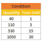
| Condition | |
| Sales Quantity | Free Unit |
| 40 | 1 |
| 110 | 3 |
| 530 | 15 |
| 1050 | 30 |
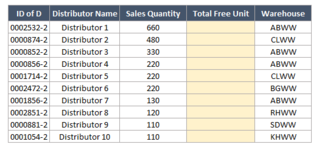
| ID of D | Distributor Name | Sales Quantity | Total Free Unit | Warehouse |
| 0002532-2 | Distributor 1 | 660 | ABWW | |
| 0000874-2 | Distributor 2 | 480 | CLWW | |
| 0000852-2 | Distributor 3 | 330 | ABWW | |
| 0000856-2 | Distributor 4 | 220 | ABWW | |
| 0001714-2 | Distributor 5 | 220 | CLWW | |
| 0002472-2 | Distributor 6 | 220 | BGWW | |
| 0001856-2 | Distributor 7 | 130 | ABWW | |
| 0002851-2 | Distributor 8 | 120 | RHWW | |
| 0000881-2 | Distributor 9 | 110 | SDWW | |
| 0001054-2 | Distributor 10 | 110 | KHWW |
| For the Sales of 3999 | ||||
| 1050 | 530 | 110 | 40 | |
| First Slab | Second Slab | Third Slab | Forth Slab | |
| Total Sales | 3150 | 530 | 220 | 80 |
| Round | 3 | 1 | 2 | 2 |
| Free Unit | 90 | 15 | 6 | 2 |
| Total Free Unit | 113 |