How can I rotate a chart 90 degree?

[yabi100]

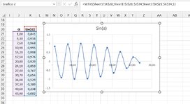
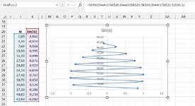
I have two columns, let say x and z of 30 points. Where z is depth and should be shown in vertical axis. And if I can show it downward, it will be perfect. I use x,y (scatter) to draw the chart which is OK but Z appears in horizontal axis but I want it to be shown in vertical axis. Simply it looks like I want to rotate the chart 90 degrees. How can I exchange z and x values in the chart?

 

[RoryA]

You can do it directly in the formula or in the Edit Series dialog:

 

[yabi100]

Can you not just edit the series and swap the X and Y ranges around?

Yes that is exactly what I want to do, but tried few things with no result. Do you mean I rearrange thier position in the Series function? I haven't tried this solution. Let me try it. In show data I clicked the buttion on top which says change but the result is not what I want and is completely wrong.

You can do it directly in the formula or in the Edit Series dialog:

View attachment 77630
I am using Excel 2016 and it is as follows:

 

[RoryA]

If that's what you see, you do not have an XY scatter series.

 

[yabi100]

If that's what you see, you do not have an XY scatter series.

Isn't this x-y scatter series?

 

[RoryA]

Yes that is an XL scatter chart but if you had an XY series selected you would have a box for x values and a box for y but you didn’t.

 

[Anthony47]

@yabi100
Another option in case the problem is still open; see the images:
-I have a serie of datas in Sheet1-J21:K34
-If I plot these datas using the scattered chart I'll get the classic curve
-now click on the curve; you will select the points on the curve, the source data will also be highlighted, and the formula associated to the curve will be shown in the formula bar
-with the given information, it will show:

=SERIE(Sheet1!$K$20;Sheet1!$J$21:$J$34;Sheet1!$K$21:$K$34;1)

Translated:

=SERIE(TheSerieName; TheHorizData; TheVerticalData; Z Position)

This is shown in the first attached image

Now if you modify that formula by exchanging TheHorizData and TheVerticalData you will get the rotated graph
As is shown in the second image

 

[yabi100]

Dear Anthony47
Just

@yabi100
Another option in case the problem is still open; see the images:
-I have a serie of datas in Sheet1-J21:K34
-If I plot these datas using the scattered chart I'll get the classic curve
-now click on the curve; you will select the points on the curve, the source data will also be highlighted, and the formula associated to the curve will be shown in the formula bar
-with the given information, it will show:

=SERIE(Sheet1!$K$20;Sheet1!$J$21:$J$34;Sheet1!$K$21:$K$34;1)

Translated:

=SERIE(TheSerieName; TheHorizData; TheVerticalData; Z Position)

This is shown in the first attached image

Now if you modify that formula by exchanging TheHorizData and TheVerticalData you will get the rotated graph
As is shown in the second image

read your answer. This is very cool and exactly is what I am looking for. Let me try it and let you know if it works for me or not?

 

[yabi100]

@yabi100
Another option in case the problem is still open; see the images:
-I have a serie of datas in Sheet1-J21:K34
-If I plot these datas using the scattered chart I'll get the classic curve
-now click on the curve; you will select the points on the curve, the source data will also be highlighted, and the formula associated to the curve will be shown in the formula bar
-with the given information, it will show:

=SERIE(Sheet1!$K$20;Sheet1!$J$21:$J$34;Sheet1!$K$21:$K$34;1)

Translated:

=SERIE(TheSerieName; TheHorizData; TheVerticalData; Z Position)

This is shown in the first attached image

Now if you modify that formula by exchanging TheHorizData and TheVerticalData you will get the rotated graph
As is shown in the second image

Dear Anthony
This wroked like a charm. Thanks for your support. I tagged your reply as: Solution

 

[Anthony47]

Thank you for the feedback