How do I count conditional formatted cells based on it's colors.

[Goldenrules]

Good day everyone and professionals in the house

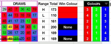
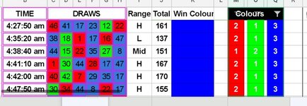
Please I really need your help with this, I have been trying to count conditional formatted cells based on it's colors, but when I didn't find the appropriate code I had to start filling it up manually.

So there are 3 major colors there Green, Red and Blue
Note (the yellow color done not count)

And anyway there is no leading color it will be referred to no winning color eg 2-2-1, 2-2-2, 3-3-0, 3-0-3.

Thanks in advance.

 

[HongRu]

Try.
My way is without VBA, but somehow complicated.
I will explain how do I get the way.
Hope this help.

Step1. To have 7 helper columns as my following XL2BB.
Step2. Put my formulas in column "I", "K:M", and "V" .
Step3. Make conditional formats in column "I".

Step1~3 just show how.
To instead, you also can copy my XL2BB into a new workbook, and add the conditional formats in column "I".

Step4. Select cell "O2" EXCATLY, and then press "Ctrl+F3" to add a new NAME "color" PRECISELY refers to "=GET.CELL(63,A2)".
Step5. Put the formula "=color" in the cell "O2".
Step6. copy the cell "O2" to cells "O2:T16".

Step4~6 should be done carefully.
If you copy from my XL2BB directly, you should just do the Step4, no more Step5~6.

And then we still have one problem.
In my example, my "RED" refers to color 3.
My "GREEN" refers to color 50.
And my "BLUE" refers to color 33.
I think we should have different RED, GREEN, or Blue very likely.

Here is my excel file to download for your reference.
color.xlsm (11.75KB) - SendSpace.com

Good luck.

color.xlsm
	A	B	C	D	E	F	G	H	I	J	K	L	M	N	O	P	Q	R	S	T	U	V
1	Draws						Range	Total	Win Color		Red	Green	Blue		Helper1	Helper2	Helper3	Helper4	Helper5	Helper6		Helper7
2											3	1	2		3	50	33	3	33	3		RED
3											4	1	1		50	33	3	3	3	3		RED
4											2	3	1		33	50	50	50	3	3		GREEN
5											3	1	2		3	50	33	3	33	3		RED
6											3	2	1		50	33	3	3	3	50		RED
7											2	3	1		33	50	50	50	3	3		GREEN
8									NONE		3	0	3		3	33	33	3	33	3
9											3	2	1		50	33	3	3	3	50		RED
10											2	3	1		33	50	50	50	3	3		GREEN
11											3	1	2		3	50	33	3	33	3		RED
12											3	2	1		50	33	3	3	3	50		RED
13											2	3	1		33	50	50	50	3	3		GREEN
14											2	1	3		3	50	33	33	33	3		BLUE
15											3	2	1		50	33	3	3	3	50		RED
16											2	3	1		33	50	50	50	3	3		GREEN
sheet1

Cell Formulas
Range	Formula
K2:K16	K2	=COUNTIF($O2:$T2,3)
L2:L16	L2	=COUNTIF($O2:$T2,50)
M2:M16	M2	=COUNTIF($O2:$T2,33)
O2:T16	O2	=color
I2:I16	I2	=IF(V2="","NONE","")
V2:V16	V2	=IF(AND(K2>L2,K2>M2),"RED","")& IF(AND(L2>K2,L2>M2),"GREEN","")& IF(AND(M2>K2,M2>L2),"BLUE","")

Cells with Conditional Formatting
Cell	Condition		Cell Format	Stop If True
I2:I16	Expression	=I2="NONE"	text	NO
I2:I16	Expression	=V2="BLUE"	text	NO
I2:I16	Expression	=V2="GREEN"	text	NO
I2:I16	Expression	=V2="RED"	text	NO

 

[Goldenrules]

Try.
My way is without VBA, but somehow complicated.
I will explain how do I get the way.
Hope this help.

Step1. To have 7 helper columns as my following XL2BB.
Step2. Put my formulas in column "I", "K:M", and "V" .
Step3. Make conditional formats in column "I".

Step1~3 just show how.
To instead, you also can copy my XL2BB into a new workbook, and add the conditional formats in column "I".

Step4. Select cell "O2" EXCATLY, and then press "Ctrl+F3" to add a new NAME "color" PRECISELY refers to "=GET.CELL(63,A2)".
Step5. Put the formula "=color" in the cell "O2".
Step6. copy the cell "O2" to cells "O2:T16".

Step4~6 should be done carefully.
If you copy from my XL2BB directly, you should just do the Step4, no more Step5~6.

And then we still have one problem.
In my example, my "RED" refers to color 3.
My "GREEN" refers to color 50.
And my "BLUE" refers to color 33.
I think we should have different RED, GREEN, or Blue very likely.

Here is my excel file to download for your reference.
color.xlsm (11.75KB) - SendSpace.com

Good luck.

color.xlsm
	A	B	C	D	E	F	G	H	I	J	K	L	M	N	O	P	Q	R	S	T	U	V
1	Draws						Range	Total	Win Color		Red	Green	Blue		Helper1	Helper2	Helper3	Helper4	Helper5	Helper6		Helper7
2											3	1	2		3	50	33	3	33	3		RED
3											4	1	1		50	33	3	3	3	3		RED
4											2	3	1		33	50	50	50	3	3		GREEN
5											3	1	2		3	50	33	3	33	3		RED
6											3	2	1		50	33	3	3	3	50		RED
7											2	3	1		33	50	50	50	3	3		GREEN
8									NONE		3	0	3		3	33	33	3	33	3
9											3	2	1		50	33	3	3	3	50		RED
10											2	3	1		33	50	50	50	3	3		GREEN
11											3	1	2		3	50	33	3	33	3		RED
12											3	2	1		50	33	3	3	3	50		RED
13											2	3	1		33	50	50	50	3	3		GREEN
14											2	1	3		3	50	33	33	33	3		BLUE
15											3	2	1		50	33	3	3	3	50		RED
16											2	3	1		33	50	50	50	3	3		GREEN
sheet1

Cell Formulas
Range	Formula
K2:K16	K2	=COUNTIF($O2:$T2,3)
L2:L16	L2	=COUNTIF($O2:$T2,50)
M2:M16	M2	=COUNTIF($O2:$T2,33)
O2:T16	O2	=color
I2:I16	I2	=IF(V2="","NONE","")
V2:V16	V2	=IF(AND(K2>L2,K2>M2),"RED","")& IF(AND(L2>K2,L2>M2),"GREEN","")& IF(AND(M2>K2,M2>L2),"BLUE","")

Cells with Conditional Formatting
Cell	Condition		Cell Format	Stop If True
I2:I16	Expression	=I2="NONE"	text	NO
I2:I16	Expression	=V2="BLUE"	text	NO
I2:I16	Expression	=V2="GREEN"	text	NO
I2:I16	Expression	=V2="RED"	text	NO

You are so amazing sir, thanks so much for your prompt response. Thanks exactly what am longing to do, you are ready a blessing to this age.

Really appreciate.

I will get to it now

 

[Goldenrules]

Try.
My way is without VBA, but somehow complicated.
I will explain how do I get the way.
Hope this help.

Step1. To have 7 helper columns as my following XL2BB.
Step2. Put my formulas in column "I", "K:M", and "V" .
Step3. Make conditional formats in column "I".

Step1~3 just show how.
To instead, you also can copy my XL2BB into a new workbook, and add the conditional formats in column "I".

Step4. Select cell "O2" EXCATLY, and then press "Ctrl+F3" to add a new NAME "color" PRECISELY refers to "=GET.CELL(63,A2)".
Step5. Put the formula "=color" in the cell "O2".
Step6. copy the cell "O2" to cells "O2:T16".

Step4~6 should be done carefully.
If you copy from my XL2BB directly, you should just do the Step4, no more Step5~6.

And then we still have one problem.
In my example, my "RED" refers to color 3.
My "GREEN" refers to color 50.
And my "BLUE" refers to color 33.
I think we should have different RED, GREEN, or Blue very likely.

Here is my excel file to download for your reference.
color.xlsm (11.75KB) - SendSpace.com

Good luck.

color.xlsm
	A	B	C	D	E	F	G	H	I	J	K	L	M	N	O	P	Q	R	S	T	U	V
1	Draws						Range	Total	Win Color		Red	Green	Blue		Helper1	Helper2	Helper3	Helper4	Helper5	Helper6		Helper7
2											3	1	2		3	50	33	3	33	3		RED
3											4	1	1		50	33	3	3	3	3		RED
4											2	3	1		33	50	50	50	3	3		GREEN
5											3	1	2		3	50	33	3	33	3		RED
6											3	2	1		50	33	3	3	3	50		RED
7											2	3	1		33	50	50	50	3	3		GREEN
8									NONE		3	0	3		3	33	33	3	33	3
9											3	2	1		50	33	3	3	3	50		RED
10											2	3	1		33	50	50	50	3	3		GREEN
11											3	1	2		3	50	33	3	33	3		RED
12											3	2	1		50	33	3	3	3	50		RED
13											2	3	1		33	50	50	50	3	3		GREEN
14											2	1	3		3	50	33	33	33	3		BLUE
15											3	2	1		50	33	3	3	3	50		RED
16											2	3	1		33	50	50	50	3	3		GREEN
sheet1

Cell Formulas
Range	Formula
K2:K16	K2	=COUNTIF($O2:$T2,3)
L2:L16	L2	=COUNTIF($O2:$T2,50)
M2:M16	M2	=COUNTIF($O2:$T2,33)
O2:T16	O2	=color
I2:I16	I2	=IF(V2="","NONE","")
V2:V16	V2	=IF(AND(K2>L2,K2>M2),"RED","")& IF(AND(L2>K2,L2>M2),"GREEN","")& IF(AND(M2>K2,M2>L2),"BLUE","")

Cells with Conditional Formatting
Cell	Condition		Cell Format	Stop If True
I2:I16	Expression	=I2="NONE"	text	NO
I2:I16	Expression	=V2="BLUE"	text	NO
I2:I16	Expression	=V2="GREEN"	text	NO
I2:I16	Expression	=V2="RED"	text	NO

Please kindly help me look into this too

Thread 'how to determine "Last Drawn" and "Mix Win Streak"' how to determine "Last Drawn" and "Mix Win Streak"