How do I dynamically create a new list from an existing list?

[russgc]

I want to build a dynamic list from an existing list.

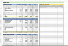
From the image you can see the list of budget items in column C. Some of those items are "savings items". Meaning I don't buy tires every month, but I want to save a little every month towards a future purchase of tires.

The list in Column I is a list I want to dynamically create from the Budget Items list in C. If you notice there is an Asterisk in column B (could be any character) that indicates if that budget item is a "savings item".

Question: How can I create a list of savings items by searching for the asterisk and populating the item and monthly savings amounts in column I, L, and M? At any time I could change any item in column B to a savings item by placing an asterisk next to the item. I would then expect the list in column I to reflect that new change.

 

[Toadstool]

Hi Russgc,

You can use AGGREGATE to retrieve each * row in turn.

Russgc.xlsx
	B	C	D	E	F	G	H	I	J	K
1
2								Marked *	1st Half	2nd Half
3	Ind	Item	1st half	2nd half	Monthly	Yearly		Tires	30	30
4		Auto Loan		400	400	4800		Oil Change	20	20
5	*	Tires	30	30	60	720		Reg	15	15
6	*	Oil Change	20	20	40	480		Clothes	22	22
7	*	Reg	15	15	30	360		Dry Cleaning	12	12
8		Gas	50	50	100	1200
9		Bus Pass			0	0
10	*	Clothes	22	22	44	528
11		Toiletries	11	11	22	264
12	*	Dry Cleaning	12	12	24	288
Sheet1

Cell Formulas
Range	Formula
I3:K12	I3	=IFERROR(INDEX(C$4:C$999,AGGREGATE(15,6,ROW($B$4:$B$999)-ROW($B$3)/($B$4:$B$999="*"),ROW()-ROW($I$2))),"")
F4:F12	F4	=SUM(D4:E4)
G4:G12	G4	=F4*12

 

[Fluff]

I suggest that you update your Account details (click your user name at the top right of the forum) so helpers always know what Excel version(s) & platform(s) you are using as the best solution often varies by version. (Don’t forget to scroll down & ‘Save’)

Another option if you have 365 & the filter function

+Fluff v2.xlsm
	A	B	C	D	E	F	G	H	I	J	K
1
2									Marked *	1st Half	2nd Half
3		Ind	Item	1st half	2nd half	Monthly	Yearly		Tires	30	30
4			Auto Loan		400	400	4800		Oil Change	20	20
5		*	Tires	30	30	60	720		Reg	15	15
6		*	Oil Change	20	20	40	480		Clothes	22	22
7		*	Reg	15	15	30	360		Dry Cleaning	12	12
8			Gas	50	50	100	1200
9			Bus Pass			0	0
10		*	Clothes	22	22	44	528
11			Toiletries	11	11	22	264
12		*	Dry Cleaning	12	12	24	288
13
14
Main

Cell Formulas
Range	Formula
I3:K7	I3	=FILTER(C4:E100,B4:B100="*")
F4:F12	F4	=SUM(D4:E4)
G4:G12	G4	=F4*12
I10:K12	I10	=IFERROR(INDEX(C$4:C$999,AGGREGATE(15,6,ROW($B$4:$B$999)-ROW($B$3)/($B$4:$B$999="*"),ROW()-ROW($I$2))),"")
Dynamic array formulas.