alm395
New Member
- Joined
- Apr 23, 2018
- Messages
- 39
- Office Version
- 365
- Platform
- Windows
Hi,
I have two separate questions.
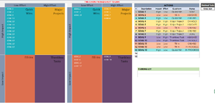
1. How would I go about having my matrix quadrants auto-populate once the quadrant is identified on the associated table? I have written several formulas, but keep receiving duplicate "Goals" appear. I have added a second matrix to my workbook to illustrate how I would like it to appear.
Formula I used
Displayed in the first matrix on the "Quick Wins" quadrant (cells C5:C19). Notice multiple duplicates.
=IF(N6="","",IF(N6="Quick Win",K6,IF(N7="","",IF(N7="Quick Win",K7,IF(N8="","",IF(N8="Quick Win",K8,IF(N9="","",IF(N9="Quick Win",K9,IF(N10="","",IF(N10="Quick Win",K10,IF(N11="","",IF(N11="Quick Win",K11,IF(N12="","",IF(N12="Quick Win",K12,IF(N13="","",IF(N13="Quick Win",K13,IF(N14="","",IF(N14="Quick Win",K14,IF(N15="","",IF(N15="Quick Win",K15,IF(N16="","",IF(N16="Quick Win",K16,IF(N17="","",IF(N17="Quick Win",K17,IF(N18="","",IF(N18="Quick Win",K18,IF(N19="","",IF(N19="Quick Win",K19,IF(N20="","",IF(N20="Quick Win",K20))))))))))))))))))))))))))))))
2. When the status changes to "DONE" on the table, I would like the associated "Goal" to remain listed on the matrix, but be crossed out. (See the attached image for "Goal 1" and "Goal 8" on the second matrix. For some reason it won't display on the XL2BB table I copied over.)
Formula I used

Thanks so much for taking time to help! This is such an amazing resource & community!!!
I have two separate questions.
1. How would I go about having my matrix quadrants auto-populate once the quadrant is identified on the associated table? I have written several formulas, but keep receiving duplicate "Goals" appear. I have added a second matrix to my workbook to illustrate how I would like it to appear.
Formula I used
Displayed in the first matrix on the "Quick Wins" quadrant (cells C5:C19). Notice multiple duplicates.
=IF(N6="","",IF(N6="Quick Win",K6,IF(N7="","",IF(N7="Quick Win",K7,IF(N8="","",IF(N8="Quick Win",K8,IF(N9="","",IF(N9="Quick Win",K9,IF(N10="","",IF(N10="Quick Win",K10,IF(N11="","",IF(N11="Quick Win",K11,IF(N12="","",IF(N12="Quick Win",K12,IF(N13="","",IF(N13="Quick Win",K13,IF(N14="","",IF(N14="Quick Win",K14,IF(N15="","",IF(N15="Quick Win",K15,IF(N16="","",IF(N16="Quick Win",K16,IF(N17="","",IF(N17="Quick Win",K17,IF(N18="","",IF(N18="Quick Win",K18,IF(N19="","",IF(N19="Quick Win",K19,IF(N20="","",IF(N20="Quick Win",K20))))))))))))))))))))))))))))))
2. When the status changes to "DONE" on the table, I would like the associated "Goal" to remain listed on the matrix, but be crossed out. (See the attached image for "Goal 1" and "Goal 8" on the second matrix. For some reason it won't display on the XL2BB table I copied over.)
Formula I used
Thanks so much for taking time to help! This is such an amazing resource & community!!!
| Matrix Test.xlsx | ||||||||||||||||||
|---|---|---|---|---|---|---|---|---|---|---|---|---|---|---|---|---|---|---|
| B | C | D | E | F | G | H | I | J | K | L | M | N | O | P | Q | |||
| 3 | THIS IS HOW I WOULD LIKE IT TO LOOK | |||||||||||||||||
| 4 | Low Effort | High Effort | Low Effort | High Effort | ACTIONS | Finished Tasks | ||||||||||||
| 5 | High Impact | GOAL 1 | High Impact | GOAL 1 | GOAL 4 | # | Description | Impact | Effort | Quadrant | Status | Cross out | ||||||
| 6 | GOAL 3 | GOAL 3 | GOAL 5 | 1 | GOAL 1 | High | Low | Quick Win | DONE | |||||||||
| 7 | GOAL 3 | GOAL 13 | GOAL 7 | 2 | GOAL 2 | Low | Low | Fill-In | ASSIGNED | |||||||||
| 8 | GOAL 13 | GOAL 8 | 3 | GOAL 3 | High | Low | Quick Win | CREATED | ||||||||||
| 9 | GOAL 13 | 4 | GOAL 4 | High | High | Major Project | ON HOLD | |||||||||||
| 10 | GOAL 13 | 5 | GOAL 5 | High | High | Major Project | ASSIGNED | |||||||||||
| 11 | GOAL 13 | 6 | GOAL 6 | Low | Low | Fill-In | CREATED | |||||||||||
| 12 | GOAL 13 | 7 | GOAL 7 | High | High | Major Project | CREATED | |||||||||||
| 13 | GOAL 13 | 8 | GOAL 8 | High | High | Major Project | DONE | |||||||||||
| 14 | GOAL 13 | 9 | GOAL 9 | Low | High | Thankless Task | ASSIGNED | |||||||||||
| 15 | GOAL 13 | 10 | GOAL 10 | Low | High | Thankless Task | ON HOLD | |||||||||||
| 16 | GOAL 13 | 11 | GOAL 11 | Low | Low | Fill-In | CREATED | |||||||||||
| 17 | GOAL 13 | 12 | GOAL 12 | Low | Low | Fill-In | IN PROGRESS | |||||||||||
| 18 | 13 | GOAL 13 | High | Low | Quick Win | IN PROGRESS | ||||||||||||
| 19 | 14 | |||||||||||||||||
| 20 | Low Impact | Low Impact | GOAL 2 | GOAL 9 | 15 | |||||||||||||
| 21 | GOAL 6 | GOAL 10 | ||||||||||||||||
| 22 | GOAL 11 | |||||||||||||||||
| 23 | GOAL 12 | |||||||||||||||||
| 24 | PARKING LOT | |||||||||||||||||
| 25 | ||||||||||||||||||
| 26 | ||||||||||||||||||
| 27 | ||||||||||||||||||
| 28 | ||||||||||||||||||
| 29 | ||||||||||||||||||
| 30 | ||||||||||||||||||
| 31 | ||||||||||||||||||
| 32 | ||||||||||||||||||
| 33 | ||||||||||||||||||
| 34 | ||||||||||||||||||
MENU (2) | ||||||||||||||||||
| Cell Formulas | ||
|---|---|---|
| Range | Formula | |
| C5:C19 | C5 | =IF(N6="","",IF(N6="Quick Win",K6,IF(N7="","",IF(N7="Quick Win",K7,IF(N8="","",IF(N8="Quick Win",K8,IF(N9="","",IF(N9="Quick Win",K9,IF(N10="","",IF(N10="Quick Win",K10,IF(N11="","",IF(N11="Quick Win",K11,IF(N12="","",IF(N12="Quick Win",K12,IF(N13="","",IF(N13="Quick Win",K13,IF(N14="","",IF(N14="Quick Win",K14,IF(N15="","",IF(N15="Quick Win",K15,IF(N16="","",IF(N16="Quick Win",K16,IF(N17="","",IF(N17="Quick Win",K17,IF(N18="","",IF(N18="Quick Win",K18,IF(N19="","",IF(N19="Quick Win",K19,IF(N20="","",IF(N20="Quick Win",K20)))))))))))))))))))))))))))))) |
| N6:N20,N25:N26 | N6 | =IF(AND(L6="",M6=""),"",(IF(AND(L6="High",M6="High"),"Major Project",IF(AND(L6="High",M6="Low"),"Quick Win",IF(AND(L6="Low",M6="High"),"Thankless Task",IF(AND(L6="Low",M6="Low"),"Fill-In")))))) |
| Cells with Conditional Formatting | ||||
|---|---|---|---|---|
| Cell | Condition | Cell Format | Stop If True | |
| G5:H34 | Expression | =AND(setting="Cross out",INDEX($J$6:$O$57,MATCH(G5,$J$6:$J$57,0),4)="DONE") | text | NO |
| J6:O34 | Expression | =$O6="DONE" | text | YES |
| C5:D34 | Expression | =AND(setting="Cross out",INDEX($J$6:$O$57,MATCH(C4,$J$6:$J$57,0),4)="DONE") | text | NO |
| J6:O34 | Expression | =$N6="Thankless Task" | text | NO |
| J6:O34 | Expression | =$N6="Fill-In" | text | NO |
| J6:O34 | Expression | =$N6="Major Project" | text | NO |
| J6:O34 | Expression | =$N6="Quick Win" | text | NO |
| Cells with Data Validation | ||
|---|---|---|
| Cell | Allow | Criteria |
| O25:O26 | List | CREATED, ASSIGNED, IN PROGRESS, ON HOLD, CANCELLED, DONE |
| O6:O20 | List | CREATED, ASSIGNED, IN PROGRESS, ON HOLD, CANCELLED, DONE |
| Q5 | List | Cross out, Remove |
| L6:M20 | List | High,Low |
| L26:M26 | List | High,Low |