How to calculate a value based on multiple criteria

[GrumpyChi]

Hi everyone,

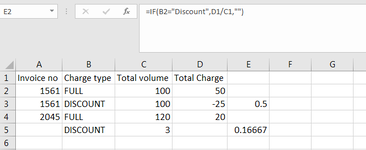
I have a data set which as an example has the below information in it


Invoice number / charge type (FULL or DISCOUNT) / Total Volume / Total Charge
1461615 FULL 100 50
1461615 DISCOUNT 100 -10
252656 FULL 150 21

So for invoice 1461615 on the discount line, I need to calculate the unit cost which is the total charge divided by the total volume but using the FULL line

I can't figure out how to do this. I've tried SUMPRODUCT but it's returning the value for the discount line unit cost which is not what I need

Thank you

 

[GrumpyChi]

Sorry the data example above did not align

Invoice no Charge type

Total volume

Total Charge

1561

FULL

100

50

1561

DISCOUNT

100

-25

2045

FULL

120

20

 

[GrumpyChi]

Can anyone help me please?

 

[Fluff]

Can anyone help me please?

Please be patient, we are all volunteers & bumping your thread 3 times in about an hour can seriously damage your chances of getting help.

In future I would recommend using the XL2BB add-in to post your data.

MrExcel has a tool called “XL2BB” that lets you post samples of your data that will allow us to copy/paste it to our Excel spreadsheets, so we can work with the same copy of data that you are. Instructions on using this tool can be found here: XL2BB Add-in

Note that there is also a "Test Here” forum on this board. This is a place where you can test using this tool (or any other posting techniques that you want to test) before trying to use those tools in your actual posts.

 

[Fluff]

Forgot to ask, will the "Full" line always be directly above the "Discount" line?

 

[GrumpyChi]

Hi, Sorry for being impatient. I appreciate that this is a volunteers forum.

The full line will usually be above the discount line, but I am not 100% sure if that will always be the case going forward.

Thank you

 

[Fluff]

Ok, how about

Fluff.xlsm
	A	B	C	D	E	F
1	Invoice no	Charge type		Total volume	Total Charge
2	1561	FULL		100	50
3	1561	DISCOUNT		100	-25	5000
4	2045	FULL		120	20
5	2045	DISCOUNT		120	-10	2400
Data

Cell Formulas
Range	Formula
F2	F2	=IF(B2="discount",PRODUCT(INDEX(D$1:E1,XMATCH(A2,A$1:A1,0,-1))),"")
F3:F5	F3	=IF(B3="discount",PRODUCT(INDEX(D$1:E2,XMATCH(A3,A$1:A2,0,-1),{1,2})),"")

 

[shinigamilight]

=IF(B2="Discount",D1/C1,"")

 

[Fluff]

Oops, misread the op.
It should be

Fluff.xlsm
	A	B	C	D	E	F
1	Invoice no	Charge type		Total volume	Total Charge
2	1561	FULL		100	50
3	1561	DISCOUNT		100	-25	0.50
4	2045	FULL		120	20
5
6	2045	DISCOUNT		120	-10	0.17
Data

Cell Formulas
Range	Formula
F2:F4	F2	=LET(m,XMATCH(A2,A$1:A1,0,-1),IF(B2="discount",INDEX(E$1:E1,m)/INDEX(D$1:D1,m),""))
F6	F6	=LET(m,XMATCH(A6,A$1:A4,0,-1),IF(B6="discount",INDEX(E$1:E4,m)/INDEX(D$1:D4,m),""))

 

[GrumpyChi]

Thank you

I (think) I have managed to come up with a formula

=IF(K603="Discount",INDEX($DN$2:$DN$687,MATCH(1,($DR$1=$K$2:$K$687)*(D603=$D$2:$D$687)*($DS$1=$L$2:$L$687),0)),"") whereby in cell DR1 and DS1 I have permanently written the words "Full" and "Standard charge". The Full and Standard charge text are in columns K & L.

D has the invoice number

I also had to create another column for the unit rate for the Full only lines where I used "IFERROR(IF(K603="Full",AL603/M603,""),"")