How to Categorize mixed data from a report like worksheet

[RafiSharif]

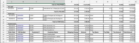
I have a worksheet that has data stored in a report like format.
Sales data with order number & other information but the issue is they are separated by country & the country name is on top of a table like structure & it repeat the same structure only the country name changes every time.
Is there anyway to have all the records in the same structure and removing the total from each country, & add the country names in a new column corresponding to the data.

 

[Toadstool]

Hi RafiSharif,

Could you post the first 20 or so rows of the report as text?

 

[RafiSharif]

Hi RafiSharif,

Could you post the first 20 or so rows of the report as text?

Here's the link to the worksheet I'm working with. dummy%20data.xlsx

 

[Toadstool]

Is that really the start of the report, because there's no Netherlands start row?

 

[RafiSharif]

Is that really the start of the report, because there's no Netherlands start row?

No that isn't the start of the spreadsheet i only have this part but the start is similar to the New Zealand section.

 

[Toadstool]

This requires that the first row of the report is a country name, like this

RafiSharif.xlsx
	A	B	C	D	E	F	G	H	I	J	K
1	NETHERLANDS
2	Order Date	SO Number	Customer #	Customer Name	Shipping Charge	Amount	Tax Name	Tax Rate	Tax Amount	Total Amount
3	12/16/2015	100005923	03084	LabID Technologies B.V.	$ 0.00	$ 1,425.00	VAT	21 %	$ 299.25	$ 1,724.25
4	12/21/2015	100005983	03452	Limgroup B.V.	$ 15.00	$ 210.40	VAT	21 %	$ 47.33	$ 272.73
5	12/23/2015	100006048	03084	LabID Technologies B.V.	$ 0.00	$ 80.70	VAT	21 %	$ 16.92	$ 97.62
6	11/10/2015	R100005013	03604	Kwekerij Piet Vijverberg B.V.	$ 0.00	$ 0.00	VAT	21 %	$ 0.00	$ 0.00
7	12/17/2015	R100005937	02096	Radboud umc	$ 0.00	$ 0.00	None	0 %	$ 0.00	$ 0.00
8	Total for NETHERLANDS:				$ 422.00	$ 14,619.35			$ 3,158.66	$ 18,200.01
9	NEW ZEALAND
10	07/09/2015	100002044	01400	Pathology Associates	$ 67.00	$ 950.17	None	0 %	$ 0.00	$ 1,017.17
11	07/21/2015	100002299	02273	Slipstream Automation	$ 65.94	$ 238.00	None	0 %	$ 0.00	$ 303.94
12	07/31/2015	100002586	01174	Canterbury District Health Board	$ 61.00	$ 720.00	None	0 %	$ 0.00	$ 781.00
Dummy Data (2)

Column N becomes a work column

RafiSharif.xlsx
	N	O	P	Q	R	S	T	U	V	W	X	Y
1			Order Date	SO Number	Customer #	Customer Name	Shipping Charge	Amount	Tax Name	Tax Rate	Tax Amount	Total Amount
2	3	NETHERLANDS	12/16/2015	100005923	03084	LabID Technologies B.V.	$ 0.00	$ 1,425.00	VAT	21 %	$ 299.25	$ 1,724.25
3	4	NETHERLANDS	12/21/2015	100005983	03452	Limgroup B.V.	$ 15.00	$ 210.40	VAT	21 %	$ 47.33	$ 272.73
4	5	NETHERLANDS	12/23/2015	100006048	03084	LabID Technologies B.V.	$ 0.00	$ 80.70	VAT	21 %	$ 16.92	$ 97.62
5	6	NETHERLANDS	11/10/2015	R100005013	03604	Kwekerij Piet Vijverberg B.V.	$ 0.00	$ 0.00	VAT	21 %	$ 0.00	$ 0.00
6	7	NETHERLANDS	12/17/2015	R100005937	02096	Radboud umc	$ 0.00	$ 0.00	None	0 %	$ 0.00	$ 0.00
7	10	NEW ZEALAND	07/09/2015	100002044	01400	Pathology Associates	$ 67.00	$ 950.17	None	0 %	$ 0.00	$ 1,017.17
8	11	NEW ZEALAND	07/21/2015	100002299	02273	Slipstream Automation	$ 65.94	$ 238.00	None	0 %	$ 0.00	$ 303.94
9	12	NEW ZEALAND	07/31/2015	100002586	01174	Canterbury District Health Board	$ 61.00	$ 720.00	None	0 %	$ 0.00	$ 781.00
10	13	NEW ZEALAND	08/11/2015	100002792	03414	GNS Science	$ 40.70	$ 50.90	None	0 %	$ 0.00	$ 91.60
11	14	NEW ZEALAND	12/01/2015	100005517	01174	Canterbury District Health Board	$ 15.00	$ 720.00	None	0 %	$ 0.00	$ 735.00
12	17	NORWAY	06/03/2015	100001111	02753	Fish Vet Group Norge AS	$ 15.00	$ 916.20	None	0 %	$ 0.00	$ 931.20
13	18	NORWAY	11/23/2015	100005358	02524	Oslo University Hospital	$ 15.00	$ 51.00	None	0 %	$ 0.00	$ 66.00
14	21	PHILIPPINES	05/20/2015	100000745	03115	Logical Form Solutions Corporation	$ 43.00	$ 200.00	None	0 %	$ 0.00	$ 243.00
Dummy Data (2)

Cell Formulas
Range	Formula
N2:N14	N2	=IFERROR(AGGREGATE(15,6,ROW($A$1:$A$9999)/(($B$1:$B$9999<>"")*($B$1:$B$9999<>"SO Number")),ROW()-ROW($P$1)),"")
O2	O2	=A1
P2:Y14	P2	=IF($N2="","",INDEX(A:A,$N2))
O3:O14	O3	=IF(N3="","",IF(AND(INDEX($B$1:$B$9999,N3-1)="",LEFT(INDEX($B$1:$B$9999,N3-1),9)<>"Total for"),INDEX($A$1:$A$9999,N3-1),O2))