Hi all,
I will try to explain this as easy as I can.
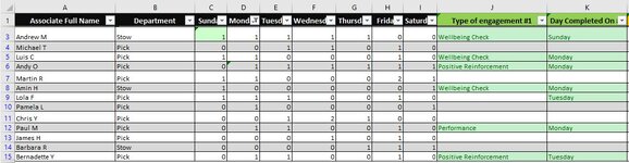
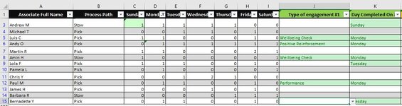
I am hoping to get some assistance on how to copy conditional formatting formula rule to cells below with their respective cell references. I am currently building a spreadsheet to track any engagement/ conversations done with employees. Column A contains employees full names. Column B contains employees department details. Columns (C to I) include every day of the week (Sunday to Saturday) and a number 1 or 0 below them. Number 1 means the employee is working on that particular day and 0 means they are not. Column J has a drop down list of every type of engagement/conversation. Column K has a drop down list including every day of the week to illustrate which specific day the engagement/conversation was completed on.
I would like Cells in Columns C to I to change colour when a value in their respective cell from column K is selected. For example, if in Cell K3 'Sunday' is selected, then C3 would turn green. This would indicate in both Cells K3 and C3 that an engagement/conversation has been completed on Sunday.
I am currently using the formula/rule =$K$3="Sunday" for cell C3 and it seems to work. However, when I copy the same formula/rule to to other cells with Format Painter, the formula doesn't change the relative reference. For example, =$K$4="Sunday" for cell C4, =$K$5="Sunday" for cell C5, etc...
I could add this formula/rule to every cell one by one but it would be time consuming. Considering there are 150+ employees.
Is there another formula I can use to get this done?
I would really appreciate some help.
Thank you!
I will try to explain this as easy as I can.
I am hoping to get some assistance on how to copy conditional formatting formula rule to cells below with their respective cell references. I am currently building a spreadsheet to track any engagement/ conversations done with employees. Column A contains employees full names. Column B contains employees department details. Columns (C to I) include every day of the week (Sunday to Saturday) and a number 1 or 0 below them. Number 1 means the employee is working on that particular day and 0 means they are not. Column J has a drop down list of every type of engagement/conversation. Column K has a drop down list including every day of the week to illustrate which specific day the engagement/conversation was completed on.
I would like Cells in Columns C to I to change colour when a value in their respective cell from column K is selected. For example, if in Cell K3 'Sunday' is selected, then C3 would turn green. This would indicate in both Cells K3 and C3 that an engagement/conversation has been completed on Sunday.
I am currently using the formula/rule =$K$3="Sunday" for cell C3 and it seems to work. However, when I copy the same formula/rule to to other cells with Format Painter, the formula doesn't change the relative reference. For example, =$K$4="Sunday" for cell C4, =$K$5="Sunday" for cell C5, etc...
I could add this formula/rule to every cell one by one but it would be time consuming. Considering there are 150+ employees.
Is there another formula I can use to get this done?
I would really appreciate some help.
Thank you!
")