How to create a dynamic check box?

[nafijmoon]

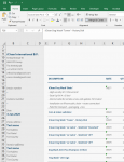
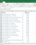
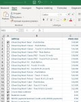
Hi. I have an excel file which has 2 sheet and so many values in there. Sheet 2 has 32 product items. And sheet 1 is my invoice. I want to add a checkbox in sheet 2 so whenever I check on an item it automatically includes in sheet 1. Serially... I attached 3 images so things get more clear.

 

[GlennUK]

Do you have your checkboxes (in your example) linked to cells in the sheet - aligned with the rows they are embedded in? Assuming that is the case ... or assuming you will do that ... you will get a TRUE or FALSE per item in the list. You then need another column of values next to those results, calculated, so as to give numbers of 1,2,3, etc for the items that are ticked. Like:
=IF(A2,COUNTIF($A$1:A2,TRUE),"")

Then, in your invoice, fetch items from the list in order, setting results to blank if there is nothing to fetch (i.e. if the ticked items have all been fetched). Using something like:
=IFNA(INDEX(Sheet2!$B$1:$B$32,MATCH(ROW()-5,Sheet2!$J$1:$J$17,0)),"")
where "ROW()-5" has been used to generate, 1 or 2 or 3 etc, as the formula is copied down (you can use whatever method to generate the pointers) .. and column J of sheet2 contains the 1,2,3 results from the previously shown formula.

Does any of that sound usable?

 

[nafijmoon]

Do you have your checkboxes (in your example) linked to cells in the sheet - aligned with the rows they are embedded in? Assuming that is the case ... or assuming you will do that ... you will get a TRUE or FALSE per item in the list. You then need another column of values next to those results, calculated, so as to give numbers of 1,2,3, etc for the items that are ticked. Like:
=IF(A2,COUNTIF($A$1:A2,TRUE),"")

Then, in your invoice, fetch items from the list in order, setting results to blank if there is nothing to fetch (i.e. if the ticked items have all been fetched). Using something like:
=IFNA(INDEX(Sheet2!$B$1:$B$32,MATCH(ROW()-5,Sheet2!$J$1:$J$17,0)),"")
where "ROW()-5" has been used to generate, 1 or 2 or 3 etc, as the formula is copied down (you can use whatever method to generate the pointers) .. and column J of sheet2 contains the 1,2,3 results from the previously shown formula.

Does any of that sound usable?

Thank you so much. I really appreciate your help.