How to Create Excel Tier List

[wchow]

Hi,

I have a set of values that need to be separate into different tier list, the values might vary from time to time but the tier list is fixed.
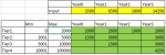
This is how it looks like:
T1: 0-2000
T2: 2001-5000
T3: 5001-10000
T4: 10001 and above
What I need to do is that let say i was given an input of 3500, then the excel formula would calculate that we have 2000 in T1 and 1500 in T2.
Please help ! Thanks in advance.

 

[Trevor G]

Welcome to the Forum,

Please can you show some sample data otherwise people would just be guessing. How is the data laid out. How do you identify a T1 compared to a T2 etc.

 

[wchow]

Hi Trevor,

Thanks for the reply. This is how it will look like:
The top input is where I key in the values, and depending on the values, they will be distributed into each tier list.
For example, i
In Year0 we have 3500, so we will get 2000 in Tier 1 and 1500 in Tier 2;
In Year1 we have 6500, so we will get 2000 in Tier 1, 3000 in Tier 2 and 1500 in Tier 3.
The yellow highlighted part will be the input from the excel user.
The green part is where the excel formula will calculate the amount of each tier based on the input the user key in.
The tier range is fixed.
Thanks again.

			Year0​	Year1​	Year2​	Year3​
		Input​	3500​	6500​	1800​	14250​
	Min​	Max​	Year0​	Year1​	Year2​	Year3​
Tier1​	0​	2000​	2000​	2000​	1800​	2000​
Tier2​	2001​	5000​	1500​	3000​		3000​
Tier3​	5001​	10000​		1500​		5000​
Tier4​	10001​	100000​				4250​

 

[wchow]

Anybody can help ?

 

[mehidy1437]

please explain for the year1 & year3

year1->tier1 2000 okay, but for tier2 you have shown 3000, but it s/b 4500 as per min & max condition. please explain the logic for this.
The same goes for year3.

 

[wchow]

please explain for the year1 & year3

year1->tier1 2000 okay, but for tier2 you have shown 3000, but it s/b 4500 as per min & max condition. please explain the logic for this.
The same goes for year3.

Hi Mehidy,

For Tier 2, the range is from 2001 to 5000, so any input above 5000 will hit the max condition of this range, and the quantity of the tier would be 3000 (5000-2000), and anything beyond that would be in Tier 3 and 4 instead.
The total of all tiers in each year should sum up to the input from the user as the formula is meant to distribute it into different tiers.

 

[Marcelo Branco]

Maybe something like this

Pasta1
	A	B	C	D	E	F	G
1				Year0	Year1	Year2	Year3
2			Input	3500	6500	1800	14250
3
4		Min	Max	Year0	Year1	Year2	Year3
5	Tier1	0	2000	2000	2000	1800	2000
6	Tier2	2001	5000	1500	3000	0	3000
7	Tier3	5001	10000	0	1500	0	5000
8	Tier4	10001	100000	0	0	0	4250
Plan7

Cell Formulas
Range	Formula
D5:G8	D5	=MAX(0,MIN(D$2-SUM(D$4:D4),$C5-$B5+IF($B5=0,0,1)))

Insert the formula in D5 copy down and across

Hope this helps

M.

 

[wchow]

Maybe something like this

Pasta1
	A	B	C	D	E	F	G
1				Year0	Year1	Year2	Year3
2			Input	3500	6500	1800	14250
3
4		Min	Max	Year0	Year1	Year2	Year3
5	Tier1	0	2000	2000	2000	1800	2000
6	Tier2	2001	5000	1500	3000	0	3000
7	Tier3	5001	10000	0	1500	0	5000
8	Tier4	10001	100000	0	0	0	4250
Plan7

Cell Formulas
Range	Formula
D5:G8	D5	=MAX(0,MIN(D$2-SUM(D$4:D4),$C5-$B5+IF($B5=0,0,1)))

Insert the formula in D5 copy down and across

Hope this helps

M.

Yeahh, thats what I needed. Thanks Marcelo !

 

[Marcelo Branco]

You are welcome. Glad to help

M.

 

[Jdogg2022]

HI Marcelo,

I have a similar issue.
I am trying to calculate when something has gone on detention.. as an example for my below table.. Days 1-7 woulod be free.. but then it goes into the next tier (8-14) which is when charges start incurring.. however it can only go to the maximum amount of days in that tier (which in this case is 7 days) before it goes to the next tier.. but keeping in mind that it is 7 days inclusive.. so once you hit 8 days of detention it should be 7 days detentention in the 8-14 catergory, and then 1 day in the 15-21 tier.

I will mention that the day to/from field has a vlookup running off it so it will change (these are already set up)
The grey box is where you would enter the amount of days detention has currently incurred.
The red cells are basically some formulars which I started to work on. But in the end saw this earlier post and thought it might be better.

Mondiale SLine Detention Rates 2022.xlsx
	O	P	Q	R
5	DAY FROM	DAY TO		Number of Days Incurred
6	8	14	8 - 14 days	7
7	15	21	15 - 21 days	6
8	22	999	22 days +	0
9
10
11			Number of days on Detention	8
Data Table New

Cell Formulas
Range	Formula
O6	O6	=VLOOKUP($S$2&$S$4&$S$3&"2",$A$2:$L$402,9,FALSE)
P6	P6	=VLOOKUP($S$2&$S$4&$S$3&"2",$A$2:$L$402,10,FALSE)
Q6	Q6	=VLOOKUP(S2,Sheet1!$A$29:$E$47,3,FALSE)
R6	R6	=IF(R11>(VLOOKUP(S2,Sheet1!$A$4:$E$17,3,FALSE)),(VLOOKUP(S2,Sheet1!$A$4:$E$17,3,FALSE)),R11)
O7	O7	=VLOOKUP($S$2&$S$4&$S$3&"3",$A$2:$L$402,9,FALSE)
P7	P7	=VLOOKUP($S$2&$S$4&$S$3&"3",$A$2:$L$402,10,FALSE)
Q7	Q7	=VLOOKUP(S2,Sheet1!$A$29:$E$47,4,FALSE)
R7	R7	=IF(R11<(N6+N7),(N7+N6)-R11,0)
O8	O8	=IF(VLOOKUP($S$2&$S$4&$S$3&"4",$A$2:$L$402,9,FALSE)="",O7,(VLOOKUP($S$2&$S$4&$S$3&"4",$A$2:$L$402,9,FALSE)))
P8	P8	=IF(VLOOKUP($S$2&$S$4&$S$3&"4",$A$2:$L$402,10,FALSE)="",P7,(VLOOKUP($S$2&$S$4&$S$3&"4",$A$2:$L$402,10,FALSE)))
Q8	Q8	=IFERROR(VLOOKUP(S2,Sheet1!$A$29:$E$47,5,FALSE),)
R8	R8	=IF(R11<O7,0,IF(AND(R11>=O7,R11<365),(R11-(R7+R6))))

Cells with Data Validation
Cell	Allow	Criteria
R7	Whole number	between 0 and N7