How to distinguish duplicates using a SORT function

ExcelColonist

New Member
Joined
Feb 1, 2021
Messages
8
Office Version
  1. 365
  2. 2019
Platform
  1. Windows
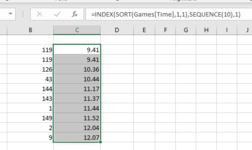
I am sorting data from a large table (called Games) for the top ten fastest running times, I will be continually adding new data to the table and the top ten times may change moving forward. I have attached a picture to be used as a visual, which also includes the function I am using.

The first column, is the table row the information is taken from
Excel Formula:
=MATCH(J2,Games[Time],0)
I eventually plan on adding an INDEX function to this equation so I can match the name to the time.

As you can see in the photo, there is a tie for first place at 9 minutes and 41 seconds, but both are sourced from the same row (row 119 in the table Games). This is the equation I am using for this.

Excel Formula:
=INDEX(SORT(Games[Time],1,1),SEQUENCE(10),1)

Both 9.41 times should be coming from their own unique rows in the table, does anyone have any ideas how I can accomplish this?
 

Attachments

  • excel1.PNG
    excel1.PNG
    13.7 KB · Views: 8

Excel Facts

Why does 9 mean SUM in SUBTOTAL?
It is because Sum is the 9th alphabetically in Average, Count, CountA, Max, Min, Product, StDev.S, StDev.P, Sum, VAR.S, VAR.P.
Match will always return the first result found (it does tell you this in the help file). For subsequent matches you need to use an array of some kind, the easiest would be something like
Excel Formula:
=IFERROR(AGGREGATE(15,6,ROW(Games[Time])/(Games[Time]=C2),COUNTIF(C$2:C2,C2))-ROW(Games[[#Headers],[Time]]),"")
Note that I've used C2 based on the screen capture as the relevance of J2 in the posted formula is not entirely clear.
 
Upvote 0
If you have the names in the table you can use something like
+Fluff 1.xlsm
ABCDEFGH
1NameTrackTime
2Tom PearceTrack 112.65Dan'l Whiddon9.26
3Bill BrewerTrack 110.37Peter Davy9.76
4Jan StewerTrack 110.69Tom Cobley9.76
5Peter GurneyTrack 214.12Bill Brewer10.37
6Peter DavyTrack 29.76Jan Stewer10.69
7Dan'l WhiddonTrack 29.26Tom Pearce12.65
8Harry HawkeTrack 314.61Peter Gurney14.12
9Tom CobleyTrack 39.76Harry Hawke14.61
Master
Cell Formulas
RangeFormula
G2:H9G2=INDEX(SORT(Table2,3,1),SEQUENCE(ROWS(Table2)),{1,3})
Dynamic array formulas.
 
Upvote 0
Match will always return the first result found (it does tell you this in the help file). For subsequent matches you need to use an array of some kind, the easiest would be something like
Excel Formula:
=IFERROR(AGGREGATE(15,6,ROW(Games[Time])/(Games[Time]=C2),COUNTIF(C$2:C2,C2))-ROW(Games[[#Headers],[Time]]),"")
Note that I've used C2 based on the screen capture as the relevance of J2 in the posted formula is not entirely clear.
J2 is the cell to the right of the cell where the fastest times are first listed, as it descends it'll be J3, J4, J5 etc until the first top ten times are listed.
 
Upvote 0
If you have the names in the table you can use something like
+Fluff 1.xlsm
ABCDEFGH
1NameTrackTime
2Tom PearceTrack 112.65Dan'l Whiddon9.26
3Bill BrewerTrack 110.37Peter Davy9.76
4Jan StewerTrack 110.69Tom Cobley9.76
5Peter GurneyTrack 214.12Bill Brewer10.37
6Peter DavyTrack 29.76Jan Stewer10.69
7Dan'l WhiddonTrack 29.26Tom Pearce12.65
8Harry HawkeTrack 314.61Peter Gurney14.12
9Tom CobleyTrack 39.76Harry Hawke14.61
Master
Cell Formulas
RangeFormula
G2:H9G2=INDEX(SORT(Table2,3,1),SEQUENCE(ROWS(Table2)),{1,3})
Dynamic array formulas.
Thank you very much, this solves my problem.

As a follow up question, if I wanted to create a MATCH function to the right of column H (column I) that returned the track number

Excel Formula:
=INDEX(Table2,MATCH(H1,Table2[Time],0),2)

It lists the tied times (9.76) both as Track 2, when one should be Track 3. What would be the method to avoid this repetition?
 
Upvote 0
How about
Excel Formula:
=INDEX(SORT(Table2,3,1),SEQUENCE(ROWS(Table2)),{1,3,2})
 
Upvote 0
Or if you just want the 10 fastest
Excel Formula:
=INDEX(SORT(Table2,3,1),SEQUENCE(10),{1,3,2})
 
Upvote 0
Solution
J2 is the cell to the right of the cell where the fastest times are first listed, as it descends it'll be J3, J4, J5 etc until the first top ten times are listed.
Actually, I'm not sure how to edit a reply, but I figured out the answer to the follow up question 10 seconds after I posted it haha.

Excel Formula:
INDEX(Table2,MATCH(H1,Table2[Name],0),2)
Easy peasy.

But what would be the solution if Peter Davy ran Track 2 AND 3 for the exact same time of 9.76. How would this be taken into account? Same runner, same time.

EDIT: found the edit button.
 
Last edited:
Upvote 0
Glad we could help & thanks for the feedback.
 
Upvote 0

Forum statistics

Threads
1,214,810
Messages
6,121,690
Members
449,048
Latest member
81jamesacct

We've detected that you are using an adblocker.

We have a great community of people providing Excel help here, but the hosting costs are enormous. You can help keep this site running by allowing ads on MrExcel.com.
Allow Ads at MrExcel

Which adblocker are you using?

Disable AdBlock

Follow these easy steps to disable AdBlock

1)Click on the icon in the browser’s toolbar.
2)Click on the icon in the browser’s toolbar.
2)Click on the "Pause on this site" option.
Go back

Disable AdBlock Plus

Follow these easy steps to disable AdBlock Plus

1)Click on the icon in the browser’s toolbar.
2)Click on the toggle to disable it for "mrexcel.com".
Go back

Disable uBlock Origin

Follow these easy steps to disable uBlock Origin

1)Click on the icon in the browser’s toolbar.
2)Click on the "Power" button.
3)Click on the "Refresh" button.
Go back

Disable uBlock

Follow these easy steps to disable uBlock

1)Click on the icon in the browser’s toolbar.
2)Click on the "Power" button.
3)Click on the "Refresh" button.
Go back
Back
Top