How to formulate a tier system

[tryingcake]

I'm not googling the right words to find this answer.

My company is implementing a new incentive payment schedule. In my first example, easy peasy. It's my second example that has me stumped.

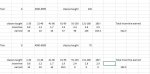
So for tier 8, if you've taught between 4,500 and 6,999 classes in your lifetime with the company, for every x amount of classes you teach this month, you get a certain amount of incentive. The incentive goes up as you teach more classes. The incentive stops rising after 180 classes taught. So if I teach 238 classes, no biggie. I can do those elementary formulas blindfolded.

However - what if they only teach 75 classes? How do I formulate each cell to give me the proper dollar amount? I can do the math in my head. How do I create a formula to do the math for me?

Thanks! please save my rear like you always do!

 

[mse330]

To make it simple, couple of helper rows added …

Book1
	A	B	C	D	E	F	G	H	I	J
1			From	1	21	41	61	91	131	181
2			To	20	40	60	90	130	180
3			Max Pts	20	20	20	30	40	50	0
4			Payout	0.8	1.2	1.7	1.9	2.4	2.6	2.9
5
6	Classes Taught	75		75	55	35	15	0	0	0
7				20	20	20	15	0	0	0
8	Dollar Amount	102.5		16	24	34	28.5	0	0	0
Sheet1

Cell Formulas
Range	Formula
E1:J1	E1	=D2+1
E2:F2	E2	=D2+20
G2	G2	=F2+30
H2	H2	=G2+40
I2	I2	=H2+50
D3:I3	D3	=D2-D1+1
J3	J3	=IF(B6-J1>0,B6-J1,0)
D6	D6	=B6
E6:J6	E6	=D6-SUM(D7)
D7:J7	D7	=IF(D6>D3,D3,D6)
D8:J8	D8	=D7*D4
B8	B8	=SUM(D8:J8)

 

[tryingcake]

Thank you! I would kiss you if I could!

 

[mse330]

Glad to help

 

[Dave Patton]

Commission2020.xlsm
	C	D	E	F	G	H
1	Number	238
2	Calculated	525.20
3	as above without named range	525.20
4	as above with arrays in formula	523.40
5
6
7		Bracket [rB]	Rate	Rate Delta [rR]	Accumulated
8		0	0.80	0.80	0.00
9		20	1.20	0.40	16.00	16.00
10		40	1.70	0.50	40.00	24.00
11		60	1.90	0.20	74.00	34.00
12		90	2.40	0.50	131.00	57.00
13		130	2.60	0.20	227.00	96.00
14		180	2.90	0.30	357.00	130.00
15		1.00E+09			525.20	168.20
16						525.20
17
18		168.20
Classes

Cell Formulas
Range	Formula
D2	D2	=SUMPRODUCT(--(D1>rB),D1-rB,rR)
D3	D3	=SUMPRODUCT(--(D1>D8:D14),D1-D8:D14,F8:F14)
D4	D4	=SUMPRODUCT(--(D1>{0;21;41;61;91;131;180}),D1-{0;21;41;61;91;131;180},{0.8;0.4;0.5;0.2;0.5;0.2;0.3})
F8:F14	F8	=E8-N(E7)
G9:G15	G9	=MAX(0,(MIN($D$1,D9)-D8))*E8+G8
H9:H15	H9	=MAX(0,(MIN($D$1,D9)-D8))*E8
H16	H16	=SUM(H9:H15)
D18	D18	=(D1-D14)*E14

Named Ranges
Name	Refers To	Cells
rB	=Classes!$D$8:$D$14	D2:D3, G9:H9
rR	=Classes!$F$8:$F$14	D2:D3

Try the approach that you prefer.
You do not need columns G & H if you use the SumProduct approach.

 

[Dave Patton]

Commission2020.xlsm
	C	D
1	Number	75
2	Calculated	102.50
3	as above without named range	102.50
Classes

Cell Formulas
Range	Formula
D2	D2	=SUMPRODUCT(--(D1>rB),D1-rB,rR)
D3	D3	=SUMPRODUCT(--(D1>{0;20;40;60;90;130;180}),D1-{0;20;40;60;90;130;180},{0.8;0.4;0.5;0.2;0.5;0.2;0.3})

This post shows the correct array in the formula; I put incorrect info in the first post.