how to have existing formula change by entering numbers into two separate cells

[drooperman]

I was wondering if someone could please help me. I have a sheet with numbers data that I am calculating through various formulas such as sums and ranges and averages and sort functions etc. My problem at the moment is that I have for instance in Column Y a set of numbers that is the main Numbers references that I entered in manually such as 1 to 10 or 4 to 19 or 19 to 29 etc. this list varies on different sheets and will never change after I have entered them the first time, as they are the main numbers. then I have the data in column Z that will change as I enter new figures into the chosen cells on other sheets. lets say for instance on sheet one these main numbers in column Y are 1 to 10. Next to each of these 1 to 10 numbers in column Z is the results of my sorting or range or xlookup formulas that I have asked for that is delivered to me. Now out of this data in column Z (next to the numbers 1 to 10), I currently have a sort formula that sorts this data into top 3 numbers for me. this sort formula is looking throughout all the 1 to 10 numbers and their accompanying data in column Z to find the top 3 numbers and then shows me the top three numbers out of 1 to 10 with its accompanying data next to it. [=SORT(FILTER(V197:W205,W197:W205>=LARGE(W197:W205, 5)), 2, -1)] The Problem I face is that sometimes this sort formula gotta be between main numbers 2 and 8 or 1 and 7 or between 3 and 9, it doesn't stay always just 1 to 10, which then requires me to manually edit the formula every time which is a lengthy process since there are over 40 columns of such data. Is there a way that I can make this formula work by me entering the start number (2) and end number (8) into two different cells which will tell this Sort formula where to start and end the top 3 numbers search? thanks in advance for all your efforts.

 

[Peter_SSs]

You're welcome. Thanks for the follow-up.

 

[drooperman]

Hi Peter,

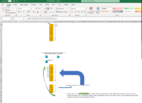
sory for bothering you again, could you maybe assist with doing the same to these three formulas. Rank/Average & XLookup.

Your help is much appreciated. thanks.

 

[Peter_SSs]

Could we get the samples with XL2BB now?

 

[drooperman]

Could we get the samples with XL2BB now?

sory peter I looked at a few videos on how to do the Xl2bb

TEST EXAMPLE 1.xlsx
	R	S	T	U	V	W	X	Y	Z	AA	AB	AC	AD	AE	AF	AG	AH	AI	AJ	AK	AL	AM	AN	AO	AP	AQ	AR	AS	AT	AU	AV	AW	AX	AY	AZ	BA	BB	BC	BD	BE	BF	BG	BH	BI	BJ	BK	BL	BM	BN
1							RANK:
2								37	8
3								38	2
4								39	6
5								40	7
6								41	5
7								42	4
8								43	3
9								44	9
10								45	10
11								46	1
12									5.5
13
14
15												AVERAGE:
16
17
18
19				ENTER FROM RANGE & TO RANGE:
20						From:				To:
21						37				45
22
23						Top Results:
24						5
25
26								37	3
27								38	9
28								39	5
29								40	4
30								41	6
31								42	7
32								43	8
33								44	2
34								45	1
35								46	10
36
37
38								38	9					Currently this gives me top 3 of ALL THESE 10
39								43	8
40								42	7
41								41	6
42								39	5
43														IF I want to get the top 3 of only NUMBERS 2 to 8 then I have to manually go in and change that formula to look only in 2 to 8.
44														Is there a way that I can just enter the FROM number in the top box to be 2 and the TO number to be 8 and then get the results
45														instead of having to keep changing the formula?
46
47
48								37	0
49								38	9
50								39	5
51								40	0	Xlookup Numbers
52								41	6
53								42	7
54								43	8
55								44	0
56								45	0
57								46	0
58
Example

Cell Formulas
Range	Formula
Y3:Y11,Y49:Y57,Y27:Y35	Y3	=Y2+1
Z2:Z11	Z2	=RANK.EQ(Z26,Z$26:Z$35)+COUNTIF(Z26,Z26)-1
Z12	Z12	=AVERAGE(Z2:Z11)
Y38:Z42	Y38	=INDEX(SORT(FILTER(Y26:Z35,(Y26:Y35>=W21)*(Y26:Y35<=AA21),""),2,-1),SEQUENCE(W24),{1,2})
Z48:Z57	Z48	=XLOOKUP(Y48,Y$38:Y$42,Z$38:Z$42,0)
Dynamic array formulas.

Hope this helps

 

[drooperman]

Could we get the samples with XL2BB now?

				RANK:
					37	8
					38	2
					39	6
					40	7
					41	5
					42	4
					43	3
					44	9
					45	10
					46	1
						5.5	AVERAGE:
	ENTER FROM RANGE & TO RANGE:
			From:				To:
			37				45
			Top Results:
			5
					37	3	This is my data Set
					38	9
					39	5
					40	4
					41	6
					42	7
					43	8
					44	2
					45	1
					46	10
					38	9	Currently this gives me top 3 of ALL THESE 10
					43	8
					42	7
					41	6
					39	5
					37	0	Xlookup Numbers
					38	9
					39	5
					40	0
					41	6
					42	7
					43	8
					44	0
					45	0
					46	0

To be clear, I want both the top Rank section, the average section below it and at the bottom the x lookup section all to change with the SORT section when I edit the FROM and TO numbers.. is this possible?

 

[Peter_SSs]

I'm not sure what the expected results are or exactly how they would be displayed.

Can you create an example where From = 41, To = 45, Top results = 4 and manually enter all the results where you would want them & post that.
Best also to get rid of all that text description about top 3 when your example is no longer about that.

 

[drooperman]

Hi Peter thanks. see this sheet is as the numbers should appear as it should be on 41 and 45 figures

See if this helps..

TEST EXAMPLE 1.xlsx
	S	T	U	V	W	X	Y	Z	AA	AB	AC	AD	AE	AF	AG
1						RANK:
2							37	8
3							38	2
4							39	6
5							40	7
6							41	3
7							42	2
8							43	1
9							44	4
10							45	5
11							46	1
12								3	AVERAGE:
13
14
15
16
17
18
19			ENTER FROM RANGE & TO RANGE:
20					From:				To:
21					41				45
22
23					Top Results:
24					4
25
26							37	3
27							38	9
28							39	5
29							40	4
30							41	6
31							42	7
32							43	8
33							44	2
34							45	1
35							46	10
36
37
38							43	8
39							42	7
40							41	6
41							44	2
42
43
44
45
46
47
48							37	0	Xlookup Numbers
49							38	0
50							39	0
51							40	0
52							41	6
53							42	7
54							43	8
55							44	2
56							45	1
57							46	0
58
Example

Cell Formulas
Range	Formula
Y3:Y11,Y49:Y57,Y27:Y35	Y3	=Y2+1
Z2:Z5,Z11	Z2	=RANK.EQ(Z26,Z$26:Z$35)+COUNTIF(Z26,Z26)-1
Z6:Z10	Z6	=RANK.EQ(Z30,Z$30:Z$34)+COUNTIF(Z30,Z30)-1
Z12	Z12	=AVERAGE(Z6:Z10)
Y38:Z41	Y38	=INDEX(SORT(FILTER(Y26:Z35,(Y26:Y35>=W21)*(Y26:Y35<=AA21),""),2,-1),SEQUENCE(W24),{1,2})
Z48:Z57	Z48	=XLOOKUP(Y48,Y$30:Y$34,Z$30:Z$34,0)
Dynamic array formulas.

 

[Peter_SSs]

Can you create an example where From = 41, To = 45, Top results = 4 and manually enter all the results where you would want them & post that.

If that is what you have now provided, then ..

In relation to RANK you already have formulas and they seem to have nothing to do with 41, 45 or 4 so if those are the results you want you are already all set.

In relation to the XLOOKUP section I have provided formulas in column Z that replicate the values in your post above and should adjust if the 41 or 45 change. Those results seemed to have nothing the do with "top 4"?
I have also provided a dynamic array formula in AB$8 that possibly may be of use.

drooperman.xlsm
	W	X	Y	Z	AA	AB	AC
20	From:				To:
21	41				45
22
23	Top Results:
24	4
25
26			37	3
27			38	9
28			39	5
29			40	4
30			41	6
31			42	7
32			43	8
33			44	2
34			45	1
35			46	10
36
37
38			43	8
39			42	7
40			41	6
41			44	2
42
43
44
45
46
47
48			37	0		41	6
49			38	0		42	7
50			39	0		43	8
51			40	0		44	2
52			41	6		45	1
53			42	7
54			43	8
55			44	2
56			45	1
57			46	0
Sheet2

Cell Formulas
Range	Formula
Y27:Y35,Y49:Y57	Y27	=Y26+1
Y38:Z41	Y38	=INDEX(SORT(FILTER(Y26:Z35,(Y26:Y35>=W21)*(Y26:Y35<=AA21),""),2,-1),SEQUENCE(W24),{1,2})
Z48:Z57	Z48	=IF(OR(Y48<W$21,Y48>AA$21),0,XLOOKUP(Y48,Y$26:Y$35,Z$26:Z$35,0))
AB48:AC52	AB48	=FILTER(Y26:Z35,(Y26:Y35>=W21)*(Y26:Y35<=AA21),"")
Dynamic array formulas.

 

[drooperman]

If that is what you have now provided, then ..

In relation to RANK you already have formulas and they seem to have nothing to do with 41, 45 or 4 so if those are the results you want you are already all set.

In relation to the XLOOKUP section I have provided formulas in column Z that replicate the values in your post above and should adjust if the 41 or 45 change. Those results seemed to have nothing the do with "top 4"?
I have also provided a dynamic array formula in AB$8 that possibly may be of use.

Hi Peter,

Thank you first and foremost for all your effort. Greatly reduced my effort that I need to manage this sheet.

The sort Solution worked great. The Xlookup set: I tried the first filter solution you provided but I needed something that kept the data in order so that
I can use the Sort solution you provided on some sheets on this specific data results, so hence why I really appreciate your dynamic array formula in AB$8.
That was exactly what I was looking for. Something that will keep the data set as it is.. this must be the same for my Rank Data

With regards to the average result underneath my Rank Data Set (Z12) I found the following solution =AVERAGEIFS(Z2:Z11,Y2:Y11,">" &AI12,Y2:Y11,"<" &AM12) but for some
reason I have to have a separate "FROM & TO" box (AI12 & AM12) that deduct 1 digit from my MAIN "FROM & ADDS 1 digit to the TO" to get the correct Average Result. I tested the
result by just using the same range on a seperate =Average formula and it wont work unless I deduct 1 digit from the "FROM" number and ADD one Digit on the "TO"
number?? just thought to share that with you and for incase someone else have the same problem in the future. If you can improve on this great otherwise it does what
I need so I am not much concerned over the Average Data Calculation Result.

As for the Rank. I still Need the Rank though. To clarify.. I want the rank to only Rank the range of whatever we enter INTO the "FROM & TO" boxes. At the moment
it ranks everything from 37 to 46. But ideally when I enter 41 and 45 I don't want it to rank 41 to 45 against all the other numbers as well. I only want 41 to 45 ranked with the rest of the
numbers ie: 37, 38, 39, 40 and 46 showing ZERO (0)
See below in Ranked Section.

Ive updated the sheet with all your previous suggestions. Its just Rank that I am trying to get as well..

TEST EXAMPLE 1.xlsx
	P	Q	R	S	T	U	V	W	X	Y	Z	AA	AB	AC	AD	AE	AF	AG	AH	AI	AJ	AK	AL	AM	AN	AO	AP	AQ	AR	AS
1
2	RANK OF DATA SET									37	0
3										38	0
4										39	0
5										40	0
6										41	3
7										42	2
8										43	1
9										44	4
10										45	5					Average FROM & TO ARRAY RANGE (DO NOT EDIT)
11										46	0									From:				To:
12										3.00	3	AVERAGE:								40				46
13
14
15
16
17
18
19						ENTER FROM RANGE & TO RANGE:
20								From:				To:
21								41				45
22
23								Top Results:
24								4
25
26				DATA SET:						37	3
27										38	9
28										39	5
29										40	4
30										41	6
31										42	7
32										43	8
33										44	2
34										45	1
35										46	10
36
37
38				DATA SET SORT						43	8
39										42	7
40										41	6
41										44	2
42
43
44
45
46
47
48				DATA SET LOOKUP						37	0
49										38	0
50										39	0
51										40	0
52										41	6
53										42	7
54										43	8
55										44	2
56										45	1
57										46	0
58
Example

Cell Formulas
Range	Formula
Z6:Z10	Z6	=RANK.EQ(Z30,Z$30:Z$34)+COUNTIF(Z30,Z30)-1
Y3:Y11,Y27:Y35	Y3	=Y2+1
Y12	Y12	=AVERAGE(Z6:Z10)
Z12	Z12	=AVERAGEIFS(Z2:Z11,Y2:Y11,">" &AI12,Y2:Y11,"<" &AM12)
AI12	AI12	=W21-1
AM12	AM12	=AA21+1
Y38:Z41	Y38	=INDEX(SORT(FILTER(Y26:Z35,(Y26:Y35>=W21)*(Y26:Y35<=AA21),""),2,-1),SEQUENCE(W24),{1,2})
Y48:Y57	Y48	=Y26
Z48:Z57	Z48	=IF(OR(Y48<W$21,Y48>AA$21),0,XLOOKUP(Y48,Y$26:Y$35,Z$26:Z$35,0))
Dynamic array formulas.

 

[Peter_SSs]

That example looks a little more like what I was expecting.
However, why do you have 45 ranked in the top section when it does not meet the "top 4 results" restriction?
If you do want that ranked, why does it get ranked 5? And what if there was more than one value not included in the "top n results"? How would you rank multiples of those?

BTW, you don't need those separate From/To values, you just need to use >= and <=

=AVERAGEIFS(Z2:Z11,Y2:Y11,">=" &W21,Y2:Y11,"<=" &AA21)