How to Highlight 'n' rows and 'n' columns, using conditional formatting

[fourdragons]

Hi,

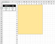
I am trying to achieve the output as shown in the image. Wanted to dynamically highlight cells based on the number of rows and columns, using conditional formatting. Given that min value is 1 and max is 50 allowed in cells E4 and F4. Please can anyone help me with this.?

Thanks in advance

 

[Fluff]

Hi & welcome to MrExcel.
How about

+Fluff 1.xlsm
	D	E	F	G	H	I	J	K	L	M	N	O	P	Q	R	S	T	U	V	W	X	Y
1								1	2	3	4	5	6	7	8	9	10	11	12	13	14	15
2							1
3							2
4		15	10				3
5							4
6							5
7							6
8							7
9							8
10							9
11							10
12							11
13							12
14							13
15							14
16							15
17							16
18							17
19							18
20							19
21							20
22							21
23							22
24							23
25							24
26							25
27							26
28							27
29							28
30							29
31							30
32							31
33							32
Main

Cell Formulas
Range	Formula
K1:BH1	K1	=SEQUENCE(,50)
J2:J51	J2	=SEQUENCE(50)
Dynamic array formulas.

Cells with Conditional Formatting
Cell	Condition		Cell Format	Stop If True
K2:BH51	Expression	=AND(ROWS(K$2:K2)<=$E$4,COLUMNS($K2:K2)<=$F$4)	text	NO

Ignore the formulae in row 1 & column J

 

[Norie]

Select K2:Y20, go to Format>Conditional formatting..., select Use formula to determine cells to format and enter this formula,

=AND(ROWS(K$2:K2)<=$E$4,COLUMNS($K2:K2)<=$F$4)

and format as required.

 

[fourdragons]

Thanks Norie

Hi & welcome to MrExcel.
How about

+Fluff 1.xlsm
	D	E	F	G	H	I	J	K	L	M	N	O	P	Q	R	S	T	U	V	W	X	Y
1								1	2	3	4	5	6	7	8	9	10	11	12	13	14	15
2							1
3							2
4		15	10				3
5							4
6							5
7							6
8							7
9							8
10							9
11							10
12							11
13							12
14							13
15							14
16							15
17							16
18							17
19							18
20							19
21							20
22							21
23							22
24							23
25							24
26							25
27							26
28							27
29							28
30							29
31							30
32							31
33							32
Main

Cell Formulas
Range	Formula
K1:BH1	K1	=SEQUENCE(,50)
J2:J51	J2	=SEQUENCE(50)
Dynamic array formulas.

Cells with Conditional Formatting
Cell	Condition		Cell Format	Stop If True
K2:BH51	Expression	=AND(ROWS(K$2:K2)<=$E$4,COLUMNS($K2:K2)<=$F$4)	text	NO

Ignore the formulae in row 1 & column J

Thank you Fluff, its working.

 

[Fluff]

Glad we could help & thanks for the feedback.

 

[fourdragons]

Select K2:Y20, go to Format>Conditional formatting..., select Use formula to determine cells to format and enter this formula,

=AND(ROWS(K$2:K2)<=$E$4,COLUMNS($K2:K2)<=$F$4)

and format as required.

Thanks Norie, its working.