How to ignore multiple cells from drag and fill or enter any formula

[Unexpc]

Hi guys

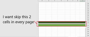
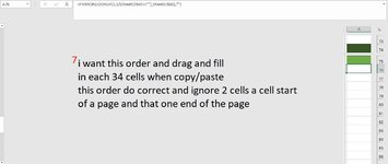
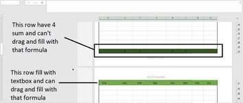
when i drag and fill, i want skip 2 rows and force not filling 2 rows (2 rows are in every page and i can't insert any formula beacuse in my workbook, all cells filling with a formula) anyway ignore this 2 rows in every page when i drag and fill? (for example i drag and fill 34 cell in 1 column and cells formula refers to a sheet cells. When i copy and paste that sheet, this 2 rows give formula that disrupting order of link cells for my page, beacuse i want this 2 specific rows 40:40,41:41 and next 34 rows ... in each page, this 2 rows should ignore from drag and fill) how solve this automate drag and fill and ignore this 2 rows?

 

[maabadi]

Try This for each 34 and 35 rows:

=IF(OR(MOD(ROW(),34)=0,MOD(ROW()-1,35)=0),"",Your Formula)

 

[Unexpc]

Try This for each 34 and 35 rows:

=IF(OR(MOD(ROW(),34)=0,MOD(ROW()-1,35)=0),"",Your Formula)

no, not work

Gofile

Gofile is a free and anonymous file-sharing platform. You can store and share data of all types (files, images, music, videos etc...). There is no limit, you download at the maximum speed of your connection and everything is free.

gofile.io

this is one of column belong my workbook please check it
i want when i copy rows 41:74 and paste in cell 75, formula in cell 76 been this: =IFERROR(LOOKUP(2,1/(Sheet1!B67<>""),Sheet1!B67),"")
and cell 74 and 75 been empty and do not drag and fill, and next 34 cell like this two....

 

[maabadi]

Check this for cell 75:
=IF(OR(MOD(ROW()-6,34)=0,MOD(ROW()-7,34)=0),"",IFERROR(LOOKUP(2,1/(Sheet1!B67<>""),Sheet1!B67),""))

and drag & fill up and down

 

[Unexpc]

Check this for cell 75:
=IF(OR(MOD(ROW()-6,34)=0,MOD(ROW()-7,34)=0),"",IFERROR(LOOKUP(2,1/(Sheet1!B67<>""),Sheet1!B67),""))

and drag & fill up and down

Show Nothing!(it is linked to Sheet1 by formula i said: =IFERROR(LOOKUP(2,1/(Sheet1!B67<>""),Sheet1!B67),"")
and i fill cells that linked but show nothing...)

 

[Unexpc]

this is what i want

 

[maabadi]

Because your source address is empty. if you have data at sheet1, it shows it. I test the file you uploaded on gofile.

 

[maabadi]

I think I understand what you want. you want to copy from sheet1 without spacing between data but paste with space. if I correct, for example if you copy sheet1!B31 to A39 , then you want to paste sheet1!B32 to A42. and this is formula ( I started this formula from A9):
=IF(OR(MOD(ROW()-6,34)=0,MOD(ROW()-7,34)=0),"",IFERROR(INDIRECT(LOOKUP(2,1/(("Sheet1!B"&ROW()-7-COUNTBLANK($A$8:A8))<>""),("Sheet1!B"&ROW()-7-COUNTBLANK($A$8:A8)))),""))

if you want to start from A8 change red parts to 6 and change Blue Parts to 7 .

 

[maabadi]

And one other thing. I assume one cell above (In this formula is A7) is empty. It is not empty add one number to red part.

 

[Unexpc]

I think I understand what you want. you want to copy from sheet1 without spacing between data but paste with space. if I correct, for example if you copy sheet1!B31 to A39 , then you want to paste sheet1!B32 to A42. and this is formula ( I started this formula from A9):
=IF(OR(MOD(ROW()-6,34)=0,MOD(ROW()-7,34)=0),"",IFERROR(INDIRECT(LOOKUP(2,1/(("Sheet1!B"&ROW()-7-COUNTBLANK($A$8:A8))<>""),("Sheet1!B"&ROW()-7-COUNTBLANK($A$8:A8)))),""))

if you want to start from A8 change red parts to 6 and change Blue Parts to 7 .

Yeah, you understand what am i want and this formula this work,im VERY THANKFUL
but i forgot say a thing
like in row 40 and next 34 row (not 41 this empty and fill with textbox), for example cell C40 i insert =sum(C8:C39) and in D40 and F40 and G40 too.
for other column no probelm with this and do correctly but this 4, i can't drag and fill your smart formula
anyway solve this problem?