How to ignore multiple cells from drag and fill or enter any formula

Unexpc

Active Member
Joined
Nov 12, 2020
Messages
496
Office Version
  1. 2019
Platform
  1. Windows
Hi guys

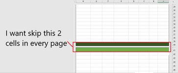
when i drag and fill, i want skip 2 rows and force not filling 2 rows (2 rows are in every page and i can't insert any formula beacuse in my workbook, all cells filling with a formula) anyway ignore this 2 rows in every page when i drag and fill? (for example i drag and fill 34 cell in 1 column and cells formula refers to a sheet cells. When i copy and paste that sheet, this 2 rows give formula that disrupting order of link cells for my page, beacuse i want this 2 specific rows 40:40,41:41 and next 34 rows ... in each page, this 2 rows should ignore from drag and fill) how solve this automate drag and fill and ignore this 2 rows?
 

Attachments

  • Screenshot 2020-11-14 165211.jpg
    Screenshot 2020-11-14 165211.jpg
    60.3 KB · Views: 59
You want hide Row of empty cells completely?!!!!
then your Page setup formula not work & your header row move up on pages.
 
Upvote 0

Excel Facts

Easy bullets in Excel
If you have a numeric keypad, press Alt+7 on numeric keypad to type a bullet in Excel.
Actually in my formula lookup is main function fot link cells from another sheet and (iferror(indirect(....))) for empty cells that not showing 0 or anything until fill and show value of linked cells and show to this cells, this my first formula =IFERROR(LOOKUP(2,1/(Sheet1!B34<>""),Sheet1!B34),"") and your solution formula =IF(MOD(ROW()-6,34)=0,SUM(C8:C39),IF(MOD(ROW()-7,34)=0,"Your Text",IFERROR(INDIRECT(LOOKUP(2,1/(("Sheet1!D"&ROW()-8-INT((ROW()-6)/34)-INT((ROW()-7)/34))<>""),("Sheet1!D"&ROW()-5-INT((ROW()-6)/34)-INT((ROW()-7)/34)))),"")))
i think when added ifferror at first formula, can be fixed
 
Upvote 0
Yes. I know. But your problem now is with indirect that return 0 result ant thus I approved the IFERROR Part to the last formula. ( 3 post before). this is complete formula:

=IF(MOD(ROW()-6,34)=0,SUM($C$8:C39),IF(MOD(ROW()-7,34)=0,"Your Text",IF(IFERROR(INDIRECT(LOOKUP(2,1/(("Sheet1!B"&ROW()-8-INT((ROW()-6)/34)-INT((ROW()-7)/34))<>""),("Sheet1!B"&ROW()-8-INT((ROW()-6)/34)-INT((ROW()-7)/34)))),"")=0,"",IFERROR(INDIRECT(LOOKUP(2,1/(("Sheet1!B"&ROW()-8-INT((ROW()-6)/34)-INT((ROW()-7)/34))<>""),("Sheet1!B"&ROW()-8-INT((ROW()-6)/34)-INT((ROW()-7)/34)))),""))))
 
Upvote 0
you are very good, this fix but show another problem
 

Attachments

  • Screenshot 2020-11-23 1252392.jpg
    Screenshot 2020-11-23 1252392.jpg
    200.4 KB · Views: 5
Upvote 0
and i before question is ( I HOPE) last question
 

Attachments

  • Screenshot 2020-11-23 124912.jpg
    Screenshot 2020-11-23 124912.jpg
    104.6 KB · Views: 4
Upvote 0
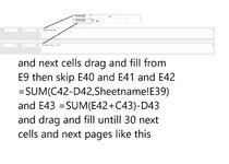
1. About Your formula, if use sum, don't use dash"-" (minus) you should remove sum and only write: =C8-D8 and ...
2. what means =Sum(C42-D42, Sheetname!E39) , Are means =C42-D42+Sheetname!E39 and Also you can Use for E43 : =C43-D43+E42
3. If you want to Skip 4 rows ( 2 Blank & 2 for your formula ) Use this (Change Red Parts with your formula):
=IF(MOD(ROW()-6,34)=0,"",IF(MOD(ROW()-7,34)=0,"",IF(MOD(ROW()-8,34)=0,C42-D42+Sheetname!E39,IF(MOD(ROW()-9,34)=0,C43-D43+E42,IF(IFERROR(INDIRECT(LOOKUP(2,1/(("Sheet1!B"&ROW()-8-INT((ROW()-6)/34)-INT((ROW()-7)/34))<>""),("Sheet1!B"&ROW()-8-INT((ROW()-6)/34)-INT((ROW()-7)/34)))),"")=0,"",IFERROR(INDIRECT(LOOKUP(2,1/(("Sheet1!B"&ROW()-8-INT((ROW()-6)/34)-INT((ROW()-7)/34))<>""),("Sheet1!B"&ROW()-8-INT((ROW()-6)/34)-INT((ROW()-7)/34)))),""))))
 
Upvote 0
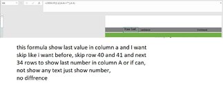
For Second Question (only show numbers):
=IF(MOD(ROW()-6,34)=0,"",IF(MOD(ROW()-7,34)=0,"",IF(ISNUMBER(LOOKUP(2,1/(A:A<>""),A:A)),LOOKUP(2,1/(A:A<>""),A:A),"")))
 
Upvote 0
1. About Your formula, if use sum, don't use dash"-" (minus) you should remove sum and only write: =C8-D8 and ...
2. what means =Sum(C42-D42, Sheetname!E39) , Are means =C42-D42+Sheetname!E39 and Also you can Use for E43 : =C43-D43+E42
3. If you want to Skip 4 rows ( 2 Blank & 2 for your formula ) Use this (Change Red Parts with your formula):
=IF(MOD(ROW()-6,34)=0,"",IF(MOD(ROW()-7,34)=0,"",IF(MOD(ROW()-8,34)=0,C42-D42+Sheetname!E39,IF(MOD(ROW()-9,34)=0,C43-D43+E42,IF(IFERROR(INDIRECT(LOOKUP(2,1/(("Sheet1!B"&ROW()-8-INT((ROW()-6)/34)-INT((ROW()-7)/34))<>""),("Sheet1!B"&ROW()-8-INT((ROW()-6)/34)-INT((ROW()-7)/34)))),"")=0,"",IFERROR(INDIRECT(LOOKUP(2,1/(("Sheet1!B"&ROW()-8-INT((ROW()-6)/34)-INT((ROW()-7)/34))<>""),("Sheet1!B"&ROW()-8-INT((ROW()-6)/34)-INT((ROW()-7)/34)))),""))))
no need skip, thanks for formula but i test and excel drag and fill correct that i want, but still showing #VALUE!
i say this thing, before i insert last formula solution for not showing empty cells, this work correctly with this simple formula but after that, it shows this error, why when you solve one my problem, a error wil be happened :(
 
Upvote 0
For Second Question (only show numbers):
=IF(MOD(ROW()-6,34)=0,"",IF(MOD(ROW()-7,34)=0,"",IF(ISNUMBER(LOOKUP(2,1/(A:A<>""),A:A)),LOOKUP(2,1/(A:A<>""),A:A),"")))
like ever, works again
 
Upvote 0
if you test =C8-D8 and it shows error because you change format cells ( at column C or D) to Text and excel don't recognize it at number.
if not please show your C8 & D8 numbers and formula that you used for see result and it show #Value Error.

and if your formula correct See this Page and change your windows setting:
How to correct a #VALUE! error
 
Upvote 0

Forum statistics

Threads
1,214,907
Messages
6,122,183
Members
449,071
Latest member
cdnMech

We've detected that you are using an adblocker.

We have a great community of people providing Excel help here, but the hosting costs are enormous. You can help keep this site running by allowing ads on MrExcel.com.
Allow Ads at MrExcel

Which adblocker are you using?

Disable AdBlock

Follow these easy steps to disable AdBlock

1)Click on the icon in the browser’s toolbar.
2)Click on the icon in the browser’s toolbar.
2)Click on the "Pause on this site" option.
Go back

Disable AdBlock Plus

Follow these easy steps to disable AdBlock Plus

1)Click on the icon in the browser’s toolbar.
2)Click on the toggle to disable it for "mrexcel.com".
Go back

Disable uBlock Origin

Follow these easy steps to disable uBlock Origin

1)Click on the icon in the browser’s toolbar.
2)Click on the "Power" button.
3)Click on the "Refresh" button.
Go back

Disable uBlock

Follow these easy steps to disable uBlock

1)Click on the icon in the browser’s toolbar.
2)Click on the "Power" button.
3)Click on the "Refresh" button.
Go back
Back
Top