How to ignore prefixes with Vlookup

[cafabrofon]

Hello,

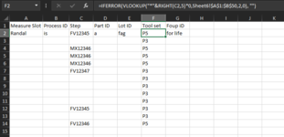
I have a formula in mind =IFERROR(VLOOKUP(A17,Sheet2!A:B,2, 0), "") the value I want to look for usually contains two letters and five numbers like FV12345 but the letters change depending on my tool set so I want to ignore the F% from the reference so that when I type the number no matter what the prefix is, it returns my tool time on the other column. so Sheet2!A contains the F%12345 and I want it to return column B. can anyone help?

 

[Saba Sabaratnam]

You can use RIGHT(A1,5) formula to ignore FV or two letters from 'Lookup value' argument.

 

[cafabrofon]

I am not sure where in the formula to plug the RIGHT(A1,5

 

[AhoyNC]

Try:

IFERROR(VLOOKUP("*"&A17,Sheet2!A:B,2, 0), "")

It is best not to reference whole columns when using the IFERROR function as this function will look at all 1 million plus rows in the worksheet which can slow down calculations.

 

[cafabrofon]

Try:

IFERROR(VLOOKUP("*"&A17,Sheet2!A:B,2, 0), "")

It is best not to reference whole columns when using the IFERROR function as this function will look at all 1 million plus rows in the worksheet which can slow down calculations.

that did not work. it returns what I want but only with specific prefix. its not ignoring the prefix

 

[JamesCanale]

How would something like this do:

MrExcelPlayground.xlsx
	A	B	C	D	E
2	Name	lookup		Table with prefix	Value
3	Harry	7		kljasdf Jamie	5
4	Jamie	5		sadjklf Fred	6
5	Fred	6		asdjlkfa Harry	7
6	John	8		asldkfj John	8
Sheet13

Cell Formulas
Range	Formula
B3:B6	B3	=INDEX($E$3:$E$6,MATCH(1,SIGN(SEARCH(A3,$D$3:$D$6))))

This isn't doing great when it finds no match for reasons I can't figure yet.

 

[Fluff]

It's not that clear what you are entering in your lookup cell, but maybe either of these

+Fluff 1.xlsm
	A	B	C	D	E
1
2	12347	C		FV12345	A
3	FV12349	E		FV12346	B
4				FV12347	C
5				FV12348	D
6				XY12349	E
7				FV12350	F
Main

Cell Formulas
Range	Formula
B2	B2	=IFNA(VLOOKUP("*"&A2,D2:E7,2,0),"")
B3	B3	=IFNA(VLOOKUP("*"&RIGHT(A3,5),D2:E7,2,0),"")

Failing that, can you post some sample data.

MrExcel has a tool called “XL2BB” that lets you post samples of your data that will allow us to copy/paste it to our Excel spreadsheets, so we can work with the same copy of data that you are. Instructions on using this tool can be found here: XL2BB Add-in

Note that there is also a "Test Here” forum on this board. This is a place where you can test using this tool (or any other posting techniques that you want to test) before trying to use those tools in your actual posts.

 

[Saba Sabaratnam]

This will be your formula if you use RIGHT formula

IFERROR(VLOOKUP(RIGHT(A17,5),Sheet2!A:B,2, 0), "")

Kind regards

Saba

 

[cafabrofon]

Thanks guys, I have the formula working like this =IFERROR(VLOOKUP("*"&RIGHT(C14,5),Sheet6!$A$1:$B$50,2,0), ""). It is finally ignoring my prefixes because of the RIGHT function. now, I can't get it to stop returning something for empty cells. what am I missing?

 

[Fluff]

How about

=IF(C14="","",IFNA(VLOOKUP("*"&RIGHT(C14,5),Sheet6!$A$1:$B$50,2,0), ""))