How to loop code that moves to next column at end and loops again, over several columns

skeeeter56

New Member
Joined
Nov 26, 2016
Messages
42
Office Version
  1. 2019
Platform
  1. Windows
I have a button when clicked runs some code which works perfect. What I want to do is when the code ends to move to next column and run again

Private Sub cbPrintUMS1_Click() Application.ScreenUpdating = False ' Get the worksheets Dim shRead As Worksheet Set shGroup1 = ThisWorkbook.Worksheets("Nunawading") Set shGroup2 = ThisWorkbook.Worksheets("Vermont") Set shGroup3 = ThisWorkbook.Worksheets("Mitcham") Set shGroup4 = ThisWorkbook.Worksheets("Blackburn") Set shGroup5 = ThisWorkbook.Worksheets("Box Hill 1") Set shGroup6 = ThisWorkbook.Worksheets("Box Hill 2") Set shData = ThisWorkbook.Worksheets("Week Commencing") 'Group1 If shData.Range("C20") = True Then ' This will copy to Nunawading Sheet shData.Range("Nuna1").Copy shGroup1.Range("D6").PasteSpecial , Paste:=xlPasteValues, Transpose:=True shGroup1.PrintPreview End If 'Group2 If shData.Range("C30") = True Then ' This will copy to Vermont Sheet shData.Range("Verm1").Copy shGroup2.Range("D6").PasteSpecial , Paste:=xlPasteValues, Transpose:=True shGroup2.PrintPreview End If 'Group3 If shData.Range("C40") = True Then ' This will copy to Mitcham Sheet shData.Range("Mitch1").Copy shGroup3.Range("D6").PasteSpecial , Paste:=xlPasteValues, Transpose:=True shGroup3.PrintPreview End If 'Group4 If shData.Range("C55") = True Then ' This will copy to Blackurn Sheet shData.Range("Black1").Copy shGroup4.Range("D6").PasteSpecial , Paste:=xlPasteValues, Transpose:=True shGroup4.PrintPreview End If 'Group5 If shData.Range("C74") = True Then ' This will copy to Box Hill 1 Sheet shData.Range("Boxh1").Copy shGroup5.Range("D6").PasteSpecial , Paste:=xlPasteValues, Transpose:=True shGroup5.PrintPreview End If 'Group6 If shData.Range("C75") = True Then ' This will copy to Box Hill 2 shData.Range("Boxhi1").Copy shGroup6.Range("D6").PasteSpecial , Paste:=xlPasteValues, Transpose:=True shGroup6.PrintPreview End If shGroup1.Range("Clear1").ClearContents shGroup2.Range("Clear2").ClearContents shGroup3.Range("Clear3").ClearContents shGroup4.Range("Clear4").ClearContents shGroup5.Range("Clear5").ClearContents shGroup6.Range("Clear6").ClearContents Application.ScreenUpdating = True End Sub


Capture.JPG


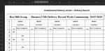
This is the Main page the rows 20,30,40,55,74 and 75 from C to P each cell has this formula =SUMPRODUCT(ISTEXT(Nuna1)+ISNUMBER(Nuna1))>0 this example checks C9:C18 to see if it contains a value gives True or False
Each Range for example in Row C20 Nuna1, D20 Nuna2 up to P20 Nuna14.
The same format is used for the other groups as it moves down the page.
Verm1 to Verm14, Mitch1 to Mitch14, Black1 to Black14, Boxh1 to Boxh14, Boxhi1 to Boxhi14

I have tried various ways to achieve but as yet have not bee able to master it. If anyone is able to help be most grateful
 

Excel Facts

How to create a cell-sized chart?
Tiny charts, called Sparklines, were added to Excel 2010. Look for Sparklines on the Insert tab.
Try this.
I guess in the destination sheet you should paste in the next available row.
If not then change this:
lr = shGroup.Cells.Find("*", , xlValues, , xlByRows, xlPrevious).Row + 1
By:
lr = 6

I grouped the data into arrays:
VBA Code:
Private Sub cbPrintUMS1_Click()
  Dim shData As Worksheet, shGroup As Worksheet
  Dim arrSh As Variant, arrCe As Variant, arrRn As Variant, arrCl As Variant
  Dim i As Long, j As Long, k As Long, lr As Long
  
  Application.ScreenUpdating = False
  arrSh = Array("Nunawading", "Vermont", "Mitcham", "Blackburn", "Box Hill 1", "Box Hill 2")
  arrCe = Array(20, 30, 40, 55, 74, 75)
  arrRn = Array("Nuna", "Verm", "Mitch", "Black", "Boxh", "Boxhi")
  arrCl = Array("Clear1", "Clear2", "Clear3", "Clear4", "Clear5", "Clear6")
  
  Set shData = ThisWorkbook.Worksheets("Week Commencing")
  For i = 0 To UBound(arrSh)
    Set shGroup = Sheets(arrSh(i))
    k = 1
    For j = Columns("C").Column To Columns("P").Column
      If shData.Cells(arrCe(i), j) = True Then
        shData.Range(arrRn(i) & k).Copy
        lr = shGroup.Cells.Find("*", , xlValues, , xlByRows, xlPrevious).Row + 1
        shGroup.Range("D" & lr).PasteSpecial , Paste:=xlPasteValues, Transpose:=True
        'shGroup.PrintPreview
      End If
      k = k + 1
    Next j
  Next i
  '
  For i = 0 To UBound(arrSh)
    Set shGroup = Sheets(arrSh(i))
    shGroup.Range(arrCl(i)).ClearContents
  Next i
  
  Application.CutCopyMode = False
  Application.ScreenUpdating = True
End Sub
 
Upvote 0
Thanks so much works perfectly and yes I have changed
lr = shGroup.Cells.Find("*", , xlValues, , xlByRows, xlPrevious).Row + 1
with
lr = 6
As the destination cells are all blank, which always starts at D6
The only issue is that when the line that Transposes the data it is changing the Font size etc, I thought that
Paste:=xlPasteValues,
would fix that.
 
Upvote 0
Already tried to put the font in the destination cells?
If you paste values, the font doesn't change, it just pastes values.
 
Upvote 0
Ok worked that out remove comma between PasteSpecial and Paste:=xlPasteValues shGroup.Range("D" & lr).PasteSpecial , Paste:=xlPasteValues, Transpose:=True
I cannot thank you enough, I wonder if you can assist again. With using the same code on another button with a slightly different code.
 
Upvote 0
This time instead of checking if a cell is True or False, I want it to see if it =2 then it precedes to do same thing but on 5 different sheets. I have changed the code
I have changed the formula that checks if the Ranges Nuna1 etc are true or false
=SUMPRODUCT(ISTEXT(Mitch3)+ISNUMBER(Mitch3))>0 with =SUMPRODUCT(ISTEXT(Mitch3)+ISNUMBER(Mitch3))>0
I need to do this as if the range is empty it is false and not sheet is printed, but as I have a another type of sheet if a certain condition is selected this is where the value 2 is used
In this case if the Range equals False and the cell in that colunm = 2 then it preceds to print, if it does not equals 2 it does not print
Also this time when it does the copy it does not need to transpose
Rich (BB code):
Private Sub cbPrintUMS1_Click()
Dim shData As Worksheet, shGroup As Worksheet
  Dim arrSh As Variant, arrCe As Variant, arrRn As Variant, arrCl As Variant
  Dim i As Long, j As Long, k As Long, lr As Long

  Application.ScreenUpdating = False

  arrSh = Array("Nunawading Bus", "Vermont Bus", "Mitcham Bus", "Blackburn Bus", "Box Hill Bus")
  arrCe = Array(21, 31, 41, 56, 75, 76)
  arrRn = Array("Nuna", "Verm", "Mitch", "Black", "Boxh", "Boxhi")
  arrCl = Array("Clear1", "Clear2", "Clear3", "Clear4", "Clear5", "Clear6")

  Set shData = ThisWorkbook.Worksheets("Week Commencing")
  For i = 0 To UBound(arrSh)
    Set shGroup = Sheets(arrSh(i))
    k = 1
    For j = Columns("C").Column To Columns("P").Column
      If shData.Cells(arrCe(i), j) = False Then
        shData.Range(arrRn(i) & k).Copy
        lr = 6
        shGroup.Range("B7").PasteSpecial
        shGroup.Range("C8").PasteSpecial
        shGroup.Range("c9").PasteSpecial
        'shGroup.PrintPreview
      End If
      k = k + 1
    Next j
  Next i

  For i = 0 To UBound(arrSh)
    Set shGroup = Sheets(arrSh(i))
    'shGroup.Range(arrCl(i)).ClearContents
  Next i

  Application.CutCopyMode = False
  Application.ScreenUpdating = True
End Sub

I have tried various ways I know that arrCe is not correct, also I have to set the range to clear these new sheets and add them as well
 
Upvote 0
In this case if the Range equals False and the cell in that colunm = 2 then it preceds to print
Column 2, but from which row?

Or you just want this:
If shData.Cells(arrCe(i), j) = 2 Then


arrSh = Array("Nunawading Bus", "Vermont Bus", "Mitcham Bus", "Blackburn Bus", "Box Hill Bus")
Are they only 5 sheets?
If there are 5 sheets, you must adjust the other 5 arrays to 5 items.
 
Upvote 0
Yes only 5 here I can fit both the data from the 2 Boxh1 to Boxhil14 range and Boxhi1 to Boxhi14 range on 1 shaeet
Sorry Row 6 Column c to P.
I will make another Range Boxhill1, Boxhill2 etc to replace both Boxh1 and Boxhi1
 
Upvote 0
Try this:

VBA Code:
If shData.Cells(arrCe(i), j) = False and  shData.Cells(6, j) = 2 Then
 
Upvote 0
Try this:

VBA Code:
If shData.Cells(arrCe(i), j) = False and  shData.Cells(6, j) = 2 Then
Yep almost there I think., just an issue where it is pasting it I think

cap2.JPG


I have added some buttons which when click change the font color and add a value to the Cell above on row 6 on each column.
I have changed the Formula for row 21, 31, 41, 56, 75, 76 from
=SUMPRODUCT(ISTEXT(Mitch1)+ISNUMBER(Mitch1))>0 to =IF(C6<>2,SUMPRODUCT(ISTEXT(Nuna1)+ISNUMBER(Nuna1))>0)
I have done this so when run the original code it does not print these as It shows False rows 21, 31, 41, 56, 75, 76 if 2 is in Cell C6 to P6
So What I need if it finds False in 21, 31, 41, 56, 75, 76 and the value in C6 to P6 =2 it then copies to these new sheets and Prints

cap.JPG


This is 1 of the new sheets they all the same format
If shData.Cells(arrCe(i), j) = False And shData.Cells(6, j) = 2 Then
If this is true it pastes the value in row 8 From Colunm C to P, value Row 9 from Colunm C to P and shData.Range(arrRn(i) & k).Copy
each loop would paste into Column s B & C, D & E, F & G, H & I , J & K.
The values from Row 8 need to be placed C4 to K4 and Row 9 C5 to K5 and original code B7, D7, F7, H7 & J7 down each of those columns
There should be no more then 5 hence why only 5 on this page, if there was more have to make it go to a new page, but maybe worry about if and when I need to
 

Attachments

  • cap.JPG
    cap.JPG
    76.4 KB · Views: 4
Upvote 0

Forum statistics

Threads
1,214,929
Messages
6,122,317
Members
449,081
Latest member
tanurai

We've detected that you are using an adblocker.

We have a great community of people providing Excel help here, but the hosting costs are enormous. You can help keep this site running by allowing ads on MrExcel.com.
Allow Ads at MrExcel

Which adblocker are you using?

Disable AdBlock

Follow these easy steps to disable AdBlock

1)Click on the icon in the browser’s toolbar.
2)Click on the icon in the browser’s toolbar.
2)Click on the "Pause on this site" option.
Go back

Disable AdBlock Plus

Follow these easy steps to disable AdBlock Plus

1)Click on the icon in the browser’s toolbar.
2)Click on the toggle to disable it for "mrexcel.com".
Go back

Disable uBlock Origin

Follow these easy steps to disable uBlock Origin

1)Click on the icon in the browser’s toolbar.
2)Click on the "Power" button.
3)Click on the "Refresh" button.
Go back

Disable uBlock

Follow these easy steps to disable uBlock

1)Click on the icon in the browser’s toolbar.
2)Click on the "Power" button.
3)Click on the "Refresh" button.
Go back
Back
Top