How to remove blank in dependent data validation dropdown list

[m_vishal_c]

HI
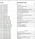
as you can see in the attached image, i need unique value for dropdown list from column A and in the second row i need the corresponding value (ignore blank) in another data validation drop down list

i.e if i select 1061 Surveyor from one dropdown list then another dropdown list will show "Surveyor", "Dream Drafting", "Atk surveying","Building professional..","Land surveying services", ïntrax consulting.."
but if i select 1011 Temprory fence then "Coates" shows blank too

i am using below formula but it shows with blank
R10 is Trade(Dropdown list)
i am applying below formula on next row to get Discipline / Trade name (but i need without blank)
=OFFSET('Supplier List'!A1,MATCH(R10,'Supplier List'!A:A,0)-1,1,COUNTIF('Supplier List'!A:A,R10))

Please guide me. i have wasted too much time but could not find .

Heaps thanks in advance

 

[maabadi]

Try Use this:

=OFFSET('Supplier List'!A1,1,MATCH(R10,'Supplier List'!A:A,0)-1,COUNTA(OFFSET('Supplier List'!A1,1,MATCH(R10,'Supplier List'!A:A,0)-1,100,1)),1)

Replace 100 with Maximum number of rows for second dropdown at source file.

For more Details Check This:
Smart Dep. Drop-Down Lists in Excel: Expandable & Exclude Blank Cells

 

[m_vishal_c]

HI Maabadi
Thanks for reply but it gives me error like "#REF!"

 

[maabadi]

Maybe you have problem with sheet name or don't update your cell references at formula with your data references.
Please upload your file with XL2BB Addin (Perferable) or upload at free uploading site, e.g. Dropbox and input link here.

 

[m_vishal_c]

Hi, Please see below link, i have uploaded file here

Temp.xlsx

Shared with Dropbox

www.dropbox.com

 

[maabadi]

I add macro to your file to Create Named Ranges at Sheet2.
Name of Main Named Range is "MainList"
For other Named Range because they cann't start with number, I add them "_" at first.
Then Select Range (Here Sheet1!E2:E118) for Trades go to Data validation select List, and at Source Box, Hit F3 and Select MainList
Then Select Range (Here Sheet1!F2) for Supplier Name go to Data validation select List, and at Source Box, and Write =indirect(E2) without $ and OK.
Check again that to Excel doesn't add to it $.
Then Drag E2 down to E118.
And at F2 write:

=IFERROR(VLOOKUP(F2,$B$2:$C$118,2,FALSE),"")

and drag it down.
Temp.xlsm

 

[m_vishal_c]

I must say a big "Thank you", just need to ask when i select _1011TEMPRORYFENCE (From E2), Unique supplier name shows 3 times "Coates", is it possible it shows unique name and column G shows different name in dropdown list
i.e E2=_1011TEMPRORYFENCE, F2="Coates"(unique), G2= all contact name in drop down list

heaps thanks

 

[maabadi]

Test This:
Temp.xlsm

 

[m_vishal_c]

sorry, it is same as before....

 

[alz]

Temp Dependent DropDown

https://sheet.zoho.com/sheet/officeapi/v1/fc223704c9f00fba6c0b6df658d5d1977ca87eec9dc249817b97dbf14cca3f83c9441147b8fee32fea87243f0a38e2b6e5fecf152f5d1dffec76c91f7e82d0b2

Hi, m_vishal_c
Check the link!