How to: Return list of values from one column based on two criteria

[AndreasMs]

Hi there,

I'm making a sheet to analyze livestream participation and want to make the document automatically list the students who are absent for a given event (chosen by drop-down menu).

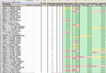
In Sheet A (see image), I have entered "Real name" of two participants. And underneath three livestream events marked them as Absent.
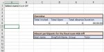
In Sheet B (see image), I want the names of any absent participant for a given livestream event to appear (can be selected using the dropdown in the top left corner).

So, using the examples in the images, if I choose Livestream event "Kick-Off", "Alibaba Story" or "PEST", I want both Andreas and Rasmus to appear as a list. And if I delete "Absent" in either of the events, the name should not appear on the list in Sheet B.

And, if, lets say, the list got 100 names on it, I want the names of those who are absent for any of those events to appear when I choose either event.

I'd then make a formula to say if "x real name" then (DingTalk Name, Group Name, Tutor) to fill in the rest based on the name that appears in the list.

I have tried with Index + Match and Lookup, but I'm not really able to figure out the logic that says: "When X event is chosen -> lookup "Absent" in Y Column -> return name in 3rd column."

Hope someone got some good ideas. I'm new to this forum, so not sure if I can upload the file if that is of any help.

Looking forward to hearing from you - thank you very much in advance!
Sincerely,
Andreas

 

[Toadstool]

Hi AndreaMs,

Here's my sample SHEET A

AndreasMs.xlsx
	C	D	E	F	G	H	I	J	K	L
2						Kick-Off	Alibaba	PEST	Soldering	Brazing
3	Real Name			# of Absent		13-Jul-20	14-Jul-20	16-Jul-20	18-Jul-20	20-Jul-20
4	Andreas			3		Absent	Absent	Absent
5	Rasmus			3		Absent	Absent	Absent
6	John			1			Absent
7	Bert			0
8	Alex			2			Absent	Absent
9	Robin			1			Absent
10	Susan			1		Absent
11	Vanessa			2		Absent	Absent
12	Hannah			0
13	James			3		Absent	Absent	Absent
14
SHEET A

Cell Formulas
Range	Formula
F4:F13	F4	=COUNTIF(H4:L4,"Absent")

Here's my SHEET B

AndreasMs.xlsx
	A	B	C	D	E	F	G
1	Select event	Kick-Off
2
7
8
9			Absent participants for the livestream Kick-Off
10			Real Name
11			Andreas
12			Rasmus
13			Susan
14			Vanessa
15			James
16
SHEET B

Cell Formulas
Range	Formula
C9	C9	="Absent participants for the livestream "&'SHEET B'!$B$1
C11:C16	C11	=IFERROR(INDEX('SHEET A'!$C$4:$C$108,AGGREGATE(15,6,ROW('SHEET A'!$H$4:$L$108)/(('SHEET A'!$H$4:$L$108<>"")*(COLUMN('SHEET A'!$H$4:$L$108)=MATCH('SHEET B'!$B$1,'SHEET A'!$H$2:$L$2,0)+COLUMN('SHEET A'!$G$1))),ROW()-ROW($C$10))-ROW('SHEET A'!$C$3)),"")

Cells with Data Validation
Cell	Allow	Criteria
B1	List	='SHEET A'!$H$2:$L$2

 

[Peter_SSs]

Welcome to the MrExcel board!

Assuming that you have the FILTER function in your Excel 365, could you use something like this?

My Sheet A

AndreasMs 2020-07-17 1.xlsm
	A	B	C	D	E	F	G	H	I	J	K	L
1
2								Kick-Off	Alibaba	PEST	Soldering	Brazing
3		Ding Talk Name	Real Name	Group Name		# of Absent		13-Jul-20	14-Jul-20	16-Jul-20	18-Jul-20	20-Jul-20
4		DTN1	Andreas	GN1		3		Absent	Absent	Absent
5		DTN2	Rasmus	GN2		3		Absent	Absent	Absent
6		DTN3	John	GN3		1			Absent
7		DTN4	Bert	GN4		0
8		DTN5	Alex	GN5		2			Absent	Absent
9		DTN6	Robin	GN6		1			Absent
10		DTN7	Susan	GN7		1		Absent
11		DTN8	Vanessa	GN8		2		Absent	Absent
12		DTN9	Hannah	GN9		0
13		DTN10	James	GN10		3		Absent	Absent	Absent
14
Sheet A

For this layout of Sheet B, the FILTER formula would need to be entered into cell C11 only. The other results would automatically 'spill' across and down to the other required cells.

AndreasMs 2020-07-17 1.xlsm
	A	B	C	D	E
1	Select event	Kick-Off
2
8
9			Absent participants for the livestream Kick-Off
10			Ding Talk Name	Real Name	Group Name
11			DTN1	Andreas	GN1
12			DTN2	Rasmus	GN2
13			DTN7	Susan	GN7
14			DTN8	Vanessa	GN8
15			DTN10	James	GN10
16
Sheet B

Cell Formulas
Range	Formula
C9	C9	="Absent participants for the livestream "&'Sheet B'!$B$1
C11:E15	C11	=FILTER('Sheet A'!B4:D200,FILTER('Sheet A'!H4:L200,'Sheet A'!H2:L2=B1)="Absent","")
Dynamic array formulas.

 

[AndreasMs]

Hi guys,

Sorry for my slow reply and thank you so much for both your time, effort and quick response. Really appreciate it!
In the end, the filter formula does the trick in the simplest way, so I end up using that one. If I may, a question in extension of that one, how do I ask it to filter Absent + e.g. those who view less than 30 minutes ("<00:30:00). I tried adding a + sign but kind really get it to work
Thank you so much for you help, truly amazing to see how quick you both respond with such detailed answers!

I got a follow up soon on the same document. Will remember to upload the full doc by then!

 

[Peter_SSs]

how do I ask it to filter Absent + e.g. those who view less than 30 minutes ("<00:30:00).

That seems to bear no relationship to what you have given us so far. You may be very familiar with your data, layout & requirement but we only have what you tell/show us. I cannot see anything that resembles "view" or time values in the images you provided.

You would need to provide some small representative sample data, the expected results (preferably with XL2BB) and explain in relation to that sample data.

 

[AndreasMs]

Hi! Yes, you are right. Sorry. Please see the two images below. I'll add Xl2BB as well for parts of it.

V2 副本 2C July September 2020 Livestream Data Template.xlsx
	A	B	C	D	E	F	G	H	I	J
2	Participants			Tutor	Attendance problems		Alibaba Story	PEST	Cainiao - Lecture	Cainiao - Interview
3	DingTalk Name	Real Name	Group Name		# of Absent	# less 1hr	07-13-2020	07-16-2020	07-21-2020	07-21-2020
4	李俊生-NPU-跨境电商-马来西亚				0	2	01:54:36	02:03:53	00:53:29	00:49:00
5	陈耀盛-NPU-跨境电商-马来西亚				0	4	00:50:34	00:00:12	00:49:34	00:50:25
6	杨欣仪-NPU-电子商务-马来西亚				0	2	01:47:36	02:00:36	00:53:35	00:51:09
7	罗曼 SHU 电子商务 俄罗斯				1	2	01:39:08	Absent	00:51:13	00:27:35
8	黄玮慷-NPU-跨境电商-马来西亚				0	2	01:54:25	01:09:10	00:52:06	00:49:58
9	蔡汶延-NPU-电商-马来西亚				0	2	01:54:58	02:03:59	00:52:45	00:48:41
10	陈勇成 NPU 电子商务 马来西亚				0	2	01:55:16	02:04:36	00:53:41	00:51:12
11	朱家仪-NPU-电子商务-马来西亚				0	2	01:54:39	02:04:16	00:52:58	00:51:09
12	黄惠忆-SHU-国贸-马来西亚				0	2	01:55:09	02:04:51	00:53:36	00:51:10
13	萧金盛-NPU-电子商务-马来西亚				1	2	Absent	02:04:44	00:53:41	00:51:13
14	龚世恩Kung Sie Ern-NPU-...				0	2	01:55:02	02:04:00	00:53:41	00:51:13
15	林悦-HIT-电子商务-马来西亚				0	2	01:55:02	02:04:05	00:53:18	00:51:06
16	梁守丰-HIT-跨境电商-马来西亚				1	2	01:54:57	Absent	00:53:10	00:51:13
17	爱玲Aizhan—SHU—电商—哈萨克斯坦				0	3	01:55:05	00:30:05	00:53:10	00:49:23
18	爱娜Aina -SHU-电子商务-哈萨克斯塔				0	2	01:27:29	01:47:17	00:51:46	00:36:28
19	陈成哲 + HIT + 电子商务+ 马来				0	2	01:54:22	02:00:57	00:53:36	00:49:51
20	沈锦升-NPU-电子商务-马来西亚				0	2	01:52:20	02:03:04	00:51:23	00:50:59
21	艾力-电子商务-NPU-俄罗斯				1	2	Absent	01:20:48	00:53:36	00:51:15
2 - Participation

Cell Formulas
Range	Formula
G2	G2	='1 - Post-Event Info Input'!$A2
H2	H2	='1 - Post-Event Info Input'!$A3
I2	I2	='1 - Post-Event Info Input'!$A4
J2	J2	='1 - Post-Event Info Input'!$A5
G3	G3	='1 - Post-Event Info Input'!$B2
H3	H3	='1 - Post-Event Info Input'!$B3
I3	I3	='1 - Post-Event Info Input'!$B4
J3	J3	='1 - Post-Event Info Input'!$B5
E4:E21	E4	=COUNTIF(G4:T4,"Absent")
F4:F21	F4	=COUNTIF(G4:T4,"<01:00:00")

Cells with Conditional Formatting
Cell	Condition		Cell Format	Stop If True
I4:J82	Cell Value	="Absent"	text	NO
I4:J82	Cell Value	<0,0208333333333333	text	NO
I4:J82	Cell Value	between 0,0208449074074074 and 0,0312384259259259	text	NO
I4:J82	Cell Value	>0,03125	text	NO
G4:G81	Cell Value	="Absent"	text	NO
G4:G81	Cell Value	between 0,0000115740740740741 and 0,0208449074074074	text	NO
G4:G81	Cell Value	between 0,0208449074074074 and 0,0416666666666667	text	NO
G4:G81	Cell Value	>0,0416666666666667	text	NO
H4:H81,G83:T90,G82:H82,K4:T82	Cell Value	="Absent"	text	NO
H4:H81,G83:T90,G82:H82,K4:T82	Cell Value	between 0,0000115740740740741 and 0,0208449074074074	text	NO
H4:H81,G83:T90,G82:H82,K4:T82	Cell Value	between 0,0208449074074074 and 0,0416666666666667	text	NO
H4:H81,G83:T90,G82:H82,K4:T82	Cell Value	>0,0416666666666667	text	NO

 

[AndreasMs]

V2 副本 2C July September 2020 Livestream Data Template.xlsx
	A	B	C	D	E	F	G
1	Select event	PEST
2
3
4			Overview
5			Total Invited	Total Open	Total Absence	Duration
6			79	76	3	00:52:02
7
8
9			Absent participants for the livestream PEST
10			DingTalk Name	Real Name	Group	Tutor
11			罗曼 SHU 电子商务 俄罗斯	0	0	0
12			梁守丰-HIT-跨境电商-马来西亚	0	0	0
13			李凯源-NPU-电子商务-马来西亚	0	0	0
14			罗君君-NPU-电子商务-马来西亚	0	0	0
15			王淇萱-NPU-跨境电商-马来西亚	0	0	0
16			张凯伊 哈工大 电商 马来西亚	0	0	0
17			杨欣悦-西工大-跨境电商-马来西亚	0	0	0
18			陈紫薇+NPU+跨境电商+马来西亚	0	0	0
19			陆志豪LOKECHEEHOU-跨境电商-NPU	0	0	0
20			赖慧珊-NPU-跨境电商-马来西亚	0	0	0
21			林慧如DISA 西工大 跨境电商 马来西亚	0	0	0
22			李欣燕-HIT-电子商务-马来西亚	0	0	0
23			蔡蕙蔚 西工大 电商 马来西亚	0	0	0
24			adam	Adam	Youth Spirit	Andreas
25			谢宁-电子商务-NPU-俄罗斯	0	0	0
26
27
28
3 - Event Analysis

Cell Formulas
Range	Formula
C6	C6	=LOOKUP($B$1,'1 - Post-Event Info Input'!$A$1:$A$17,'1 - Post-Event Info Input'!$D$1:$D$17)
D6	D6	=LOOKUP($B$1,'1 - Post-Event Info Input'!$A$1:$A$17,'1 - Post-Event Info Input'!$E$1:$E$17)
E6	E6	=LOOKUP($B$1,'1 - Post-Event Info Input'!$A$1:$A$17,'1 - Post-Event Info Input'!$F$1:$F$17)
F6	F6	=LOOKUP($B$1,'1 - Post-Event Info Input'!$A$1:$A$17,'1 - Post-Event Info Input'!$C$1:$C$17)
C9	C9	="Absent participants for the livestream "&B1
C11:F25	C11	=FILTER('2 - Participation'!A4:D90,FILTER('2 - Participation'!G4:T90,'2 - Participation'!G2:T2=B1)="Absent","")
Dynamic array formulas.

 

[Peter_SSs]

I'm not sure I have understood correctly but is this it?

=FILTER('2 - Participation'!A4:D90,(FILTER('2 - Participation'!G4:T90,'2 - Participation'!G2:T2=B1)="Absent")+(FILTER('2 - Participation'!G4:T90,'2 - Participation'!G2:T2=B1)<1/48)*(FILTER('2 - Participation'!G4:T90,'2 - Participation'!G2:T2=B1)<>""),"")