How to simplify a nested "IF" formula with a test & reference to multiple VLOOKUP tables?

FlummoxedByExcel

New Member
Joined
Jun 1, 2021
Messages
15
Office Version
  1. 365
Platform
  1. MacOS
Hi Excel geniuses, I'm looking for help simplifying this ugly (but working!) formula.
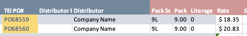
First it performs a test to see if a PO is over or under a certain number. (Thank you @Peter_SSs and @etaf !)
Based on that PO Number, I direct the next calculations to one of two VLOOKUP tables — one has old pricing, one has new pricing.
The VLOOKUP tables contain a list of customers in column A. Cols B - T in the customer name row are prices for different box sizes, which vary by customer.
My worksheet first looks for the box size in Col. I, then the customer name in Column E. It finds an exact match for the customer and the box size in the VLOOKUP table, then pulls the box price from the correct column. I'd like to find a way to avoid all this repetition if possible. Thanks to anyone who can help! I did try "IFS" but it returned an error.
(The formula is actually much longer than this as there are many more box sizes! I cut it down for clarity)
=IF(RIGHT(C3,5)*1>=68560,
IF(I4="9L",VLOOKUP(E4,Rules_NY!A:T,2,FALSE),
IF(I4="retail",VLOOKUP(E4,Rules_NY!A:T,2,FALSE),
IF(I4="4.5L",VLOOKUP(E4,Rules_NY!A:T,3,FALSE),
IF(I4="20L",VLOOKUP(E4,Rules_NY!A:T,4,FALSE),
IF(I4="12L",VLOOKUP(E4,Rules_NY!A:T,5,FALSE),
IF(I4="8L",VLOOKUP(E4,Rules_NY!A:T,6,FALSE),
)))))),
IF(I4="9L",VLOOKUP(E4,Rules_N19Y!A:T,2,FALSE),
IF(I4="retail",VLOOKUP(E4,Rules_N19Y!A:T,2,FALSE),
IF(I4="4.5L",VLOOKUP(E4,Rules_N19Y!A:T,3,FALSE),
IF(I4="20L",VLOOKUP(E4,Rules_N19Y!A:T,4,FALSE),
IF(I4="12L",VLOOKUP(E4,Rules_N19Y!A:T,5,FALSE),
IF(I4="8L",VLOOKUP(E4,Rules_N19Y!A:T,6,FALSE),
)))))))
 

Excel Facts

Bring active cell back into view
Start at A1 and select to A9999 while writing a formula, you can't see A1 anymore. Press Ctrl+Backspace to bring active cell into view.
This should produce the same result as formula above i think!

=VLOOKUP(E4,CHOOSE((0+RIGHT(C3,5)>=68560)+1,Rules_N19Y!A:T,Rules_NY!A:T),VLOOKUP(I4,{"12L",5;"20L",4;"4.5L",3;"8L",6;"9L",2;"retail",2},2,0),0)
 
Upvote 0
Solution
You can create a named range, for example "boxsizes" with the following data
varios 11oct2021.xlsm
LM
2box sizesColumn
39L2
4retail2
54.5L3
620L4
712L5
88L6
Sheet1

How to name a range:

So the formula could be:

Dante Amor
ACEIJ
1
2POCustomerBox SizePrice
3a68580
4dan4.5L101
5
6
7
Sheet1
Cell Formulas
RangeFormula
J4J4=VLOOKUP(E4,IF(RIGHT(C3,5)*1>=68560,Rules_NY!A:T,Rules_N19Y!A:T),VLOOKUP(I4,boxsizes,2,0),0)
Named Ranges
NameRefers ToCells
boxsizes=Sheet1!$L$2:$M$8J4
 
Upvote 0
Unless your issue has already resolved, it would make it much easier for us to test something if we had some sample data (& expected results) with XL2BB so that we did not have to try to 'reverse engineer' your long formula to try to work out exactly what you data is like. :)
 
Upvote 0
Thanks @steve the fish — I'm a basic excel user & learning new things from this forum. Please indulge — it looks like you re-arranged my formula and I want to understand how it works so I can continue to modify. I haven't used the CHOOSE function before.
=VLOOKUP(E4,
[E4 is the name of the customer: Excel stores the name of the customer]

CHOOSE((0+RIGHT(C3,5)>=68560)+1,
Rules_N19Y!A:T,
Rules_NY!A:T),
[Excel then looks at the PO number and tests the value. Based on the value, I think you're directing Excel to one of two VLOOKUP tables depending on if the PO is ≥68560. I don't understand the syntax though]

VLOOKUP(I4,{"12L",5;"20L",4;"4.5L",3;"8L",6;"9L",2;"retail",2},2,0),0)
[once Excel goes to the correct VLOOKUP table it will use the stored customer name to find the customer, then pull the value from I4 to lookup the correct price. It will apply this same instruction to whatever VLOOKUP table it goes to]

The VLOOKUP tables are set up exactly the same, so a value in one would be in the same spot as the value in the other one, although the pricing is different. But can a single VLOOKUP be used in multiple tables?

@DanteAmor I think your solution might work except that there are a couple hundred customers, 5 different pricing levels and a dozen box sizes, and the VLOOKUP tables are already set up years back, so I have to work within those parameters.
 
Upvote 0
I want to understand how it works so I can continue to modify
The values in that final VLOOKUP simply match the values you used to direct the VLOOKUP to the correct column based on the size . So continue to add the size and column number in pairs into that VLOOKUP as steve the fish has done. Each pair has a comma between the 2 values and each pair is separated by a semicolon.

VLOOKUP(I4,{"12L",5;"20L",4;"4.5L",3;"8L",6;"9L",2;"retail",2}

IF(I4="9L",VLOOKUP(E4,Rules_NY!A:T,2,FALSE),
IF(I4="retail",VLOOKUP(E4,Rules_NY!A:T,2,FALSE),
IF(I4="4.5L",VLOOKUP(E4,Rules_NY!A:T,3,FALSE),
IF(I4="20L",VLOOKUP(E4,Rules_NY!A:T,4,FALSE),
 
Upvote 0
thank you @Peter_SSs is there a way to have Excel look up the customer name (E4) first and then store the value so I don't have to repeat it like this: IF(I4="9L",VLOOKUP(E4,Rules_NY!A:T,2,FALSE) for every box size? I am not sure if in @steve the fish 's solution it stores the value? Basically I am not sure I can store the customer name value, then test the PO#, then branch out to one of two VLOOKUPS and recall the customer name — I dont see in the formula where it's recalled — then pull the box size. Current formula pulls the box size first then matches the customer name and directs to the correct cell on the same row for the box price. Sorry to be so dense! I am learning how this works.
The VLOOKUP solution you provided is very elegant, thanks, I am just trying to figure out how to use it!
 
Upvote 0
is there a way to have Excel look up the customer name (E4) first and then store the value so I don't have to repeat it like this: IF(I4="9L",VLOOKUP(E4,Rules_NY!A:T,2,FALSE) for every box size?
The formulas proposed by @steve the fish and @DanteAmore do not require you to repeat the customer name (E4), it just appears once in each formula.

=VLOOKUP(E4,CHOOSE((0+RIGHT(C3,5)>=68560)+1,Rules_N19Y!A:T,Rules_NY!A:T),VLOOKUP(I4,{"12L",5;"20L",4;"4.5L",3;"8L",6;"9L",2;"retail",2},2,0),0
=VLOOKUP(E4,IF(RIGHT(C3,5)*1>=68560,Rules_NY!A:T,Rules_N19Y!A:T),VLOOKUP(I4,boxsizes,2,0),0)

The basic difference between the formulas is that the first one lists all the box size/column numbers in the formula itself, whereas the second one stores those pairings somewhere in your workbook rather than in the formula.

Have you tried either of them?
 
Upvote 0
thanks @Peter_SSs , Dante's formula would have required me to recreate the vlookup table, which doesn't make sense at this time — although it will be simplified soon, so I may be able to use that solution in the future. I don't see the branch in either one of them — based on the PO# the VLookup has to branch to one of two tables. My ugly formula does do that correctly, albeit with a lot of repetition. I uploaded 2 images. In the "Results Page" the formula sits in the "rate" column and returns the correct price by using the PO# from Col C to choose which Vlookup table to reference; the Customer Name in Col E to pick the right row in the table, and the pack size in Col I to pick the correct cell in that row. The cutoff PO# is 68560, and you see my formula returns different prices for the 9L pack size of "Company Name" PO68559 & PO68560.
2nd image is a row in one of the VLookup tables where the pricing is pulled. Honestly probably not worth a lot more (if any more) of your time! but thanks for all the help provided!
 

Attachments

  • Vlookup price table.png
    Vlookup price table.png
    35.2 KB · Views: 13
  • results page.png
    results page.png
    31.1 KB · Views: 14
Upvote 0

Forum statistics

Threads
1,214,375
Messages
6,119,168
Members
448,870
Latest member
max_pedreira

We've detected that you are using an adblocker.

We have a great community of people providing Excel help here, but the hosting costs are enormous. You can help keep this site running by allowing ads on MrExcel.com.
Allow Ads at MrExcel

Which adblocker are you using?

Disable AdBlock

Follow these easy steps to disable AdBlock

1)Click on the icon in the browser’s toolbar.
2)Click on the icon in the browser’s toolbar.
2)Click on the "Pause on this site" option.
Go back

Disable AdBlock Plus

Follow these easy steps to disable AdBlock Plus

1)Click on the icon in the browser’s toolbar.
2)Click on the toggle to disable it for "mrexcel.com".
Go back

Disable uBlock Origin

Follow these easy steps to disable uBlock Origin

1)Click on the icon in the browser’s toolbar.
2)Click on the "Power" button.
3)Click on the "Refresh" button.
Go back

Disable uBlock

Follow these easy steps to disable uBlock

1)Click on the icon in the browser’s toolbar.
2)Click on the "Power" button.
3)Click on the "Refresh" button.
Go back
Back
Top