How to solve for this?

[sunnykaw]

Hello,

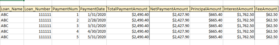
I am trying to solve for a loan amortizing schedule to be able to give an output in the next tab for all the payments to give a cumulative value based on the date.
How can I achieve this to reflect cumulative payments for July 31st or Jan 31st of each year?

 

[kweaver]

Welcolme to Mr. Excel,

Something like this, if I understand what you want to accomplish?

Book1
	A	B	C	D	E	F	G	H
1	PV	100000		Month	Date		Cum until	10/1/2021
2	Annual Rate	8%		1	1/1/2021		($7,527.96)
3	Years	20		2	2/1/2021
4	Mo'ly Pmt	($836.44)		3	3/1/2021
5				4	4/1/2021
6				5	5/1/2021
7				6	6/1/2021
8				7	7/1/2021
9				8	8/1/2021
10				9	9/1/2021
11				10	10/1/2021
12				11	11/1/2021
13				12	12/1/2021
14				13	1/1/2022
15				14	2/1/2022
16				15	3/1/2022
Sheet9

Cell Formulas
Range	Formula
G2	G2	=$B$4*DATEDIF(E2,H1,"M")
B4	B4	=PMT(B2/12,B3*12,B1)
E3:E16	E3	=EDATE(E2,1)

 

[sunnykaw]

Thanks for this solution. Unfortunately that's not what I am trying to accomplish. I am trying to get an output from the original data that I uploaded the picture. The solution needs a page where I can put in the deal name/number and select the date I want and the solution would give me an array of all cumulative amounts before that date for that particular loan into different rows. The rows as defined in my picture.

For example: I want to see all the payments made for a particular deal uptill 1/311/2021.

Loan_Name

Loan_Number

PaymentNum

PaymentDate

TotalPayment Amount

NetPaymentAmount

PrincipalAmount

InterestAmount

FeeAmount

 

[kweaver]

I can't tell from your image what the loan was (i.e., PV, rate, # payments).
Also, if you would use XL2BB no one trying to help would have to try to recreate your data.

Have you explored functions such as PMT, IPMT, PPMT, etc.?

 

[kweaver]

I made up some numbers for a loan. Is this what you're trying to find? If not, please provide more information. Thanks.

Book1
	A	B	C	D	E	F	G	H	I	J	K
1	Loan	Loan #	PaymentNum	Date	Total Amt	Net Amt	PrinAmt	IntAmt	Fee Amt	Cum Prin	Cum Int
2	ABC	111111	1	1/31/2020	$2,684.11	$2,621.61	$600.77	$2,083.33	$62.50	$600.77	$2,083.33
3	ABC	111111	2	2/28/2020	$2,684.11	$2,621.61	$603.28	$2,080.83	$62.50	$1,204.05	$4,164.16
4	ABC	111111	3	3/31/2020	$2,684.11	$2,621.61	$605.79	$2,078.32	$62.50	$1,809.84	$6,242.48
5	ABC	111111	4	4/30/2020	$2,684.11	$2,621.61	$608.32	$2,075.79	$62.50	$2,418.16	$8,318.27
6	ABC	111111	5	5/31/2020	$2,684.11	$2,621.61	$610.85	$2,073.26	$62.50	$3,029.01	$10,391.53
Sheet11

Cell Formulas
Range	Formula
E2:E6	E2	=-PMT(5%/12,30*12,500000)
F2:F6	F2	=E2-I2
G2:G6	G2	=-PPMT(5%/12,C2,12*30,500000)
H2:H6	H2	=-IPMT(5%/12,C2,12*30,500000)
J2:J6	J2	=SUM($G$2:G2)
K2:K6	K2	=SUM($H$2:H2)