How to sort 2 columns in order?

[danbates]

Hi,

Please can someone help me?

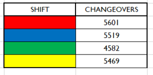
I am trying to sort 2 columns in order. Column F has values in generated by formulas and column E has a coloured cells.

What I would like is column F to sort in ascending order and column E to sort with it so the values before it sorts are still next the the right coloured cells after it has sorted.

Thanks
Dan

 

[jasonb75]

If you sort with both columns selected then it might work. It would definitely work if you didn't have formulas in the second column, but some formulas don't play well with sorting.

 

[danbates]

Hi,
yeah I've tried that but it doesn't give me the correct order. It just swaps the green and yellow cells.

I have just tried copying the numbers and then pasting them in the same location as numbers and that works.

Don't you think there is any way around this without converting the formulas to actual numbers?

 

[jasonb75]

Don't you think there is any way around this without converting the formulas to actual numbers?

I think that it is unlikely, but without knowing what the formulas are, or where they are pulling the values from it is impossible to say.

 

[kennypete]

This works for simple formulas in the Col F cells provided you are happy adding text of the same colour to the Col E cells (or I guess it could be deleted after):

Sub SortColour()
    Dim n As Integer
    Dim c As Integer
    Dim d As Object
    Set d = CreateObject("Scripting.Dictionary")

    For n = 2 To 5
        Cells(n, 5) = Cells(n, 6).Value
        c = Range("E" & Trim(Str(n))).Interior.ColorIndex
        Range("E" & Trim(Str(n))).Font.ColorIndex = c
        d.Add Key:=Range("E" & Trim(Str(n))).Value, Item:=Range("F" & Trim(Str(n))).Formula
    Next n
    Sheet1.Sort.SortFields.Clear
    Sheet1.Sort.SortFields.Add2 Key:=Range("E2:E5") _
        , SortOn:=xlSortOnValues, Order:=xlAscending, DataOption:=xlSortNormal
    With ActiveWorkbook.Worksheets("Sheet1").Sort
        .SetRange Range("E2:F5")
        .Header = xlGuess
        .Apply
    End With
    For n = 2 To 5
        Range("F" & Trim(Str(n))).Formula = d(Cells(n, 5).Value)
    Next n

End Sub

Note it's only for the E2:F5 range, but could obviously be extended. Note too it relies on the values being unique.
Input:

Book2
	E	F	G	H
2		2	5	3
3		3	4	1
4		4	3	-1
5		1	5	4
Sheet1

Cell Formulas
Range	Formula
F2:F5	F2	=G2-H2

Output:

Book2
	E	F	G	H
2	1	1	5	3
3	2	2	4	1
4	3	3	3	-1
5	4	4	5	4
Sheet1

Cell Formulas
Range	Formula
F2	F2	=G5-H5
F3:F5	F3	=G2-H2

 

[danbates]

Hi,

I've managed to sort it luckily. The problem I had is that I hadn't made all my cell references in the formulas obsolute.

Thank you very much for your help and suggestions, I do appreciate you helping me.

Thanks

Dan