How to sum values in column D until a blank cell is reached and if values in column C equals "WP" or "BS"

jfin1ty

New Member
Joined
May 15, 2023
Messages
23
Office Version
  1. 365
Platform
  1. Windows
Hi everyone,
I'm hoping you can help me with an excel formula to solve a problem I'm stuck on.
I think I am pretty close to solution but just can't crack what it is I need to make the formula work how I would like.
Basically, the problem is this:
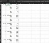
My formula is pasted all down column B. I need to sum all the values in column D up until a blank cell is reached. On top of this, I only want it to sum the values in column D until a blank cell is reached in column C and only if the values in column C equal "WP" or "BS". If a value in column C equals anything else, then I don't need it added to the sum of column D.
To round it all off, I need it to only sum the values in column D is column A is not blank.

I got as far as the below, but this formula just counts all values in column D until a blank cell is reached as long as the value in column A is not blank.
=IF(A1<>"",SUM(D1:INDEX(D1:$D$1000,MATCH(TRUE,(D2:$D$1000=""),0))),"")

I need to incorporate this formula into a sheet that doesn't really have room for helper columns and the like so if its possible to work it into one formula to copy down the whole B column that would be great.
 

Attachments

  • Excel Formula.JPG
    Excel Formula.JPG
    78.4 KB · Views: 30

Excel Facts

Format cells as currency
Select range and press Ctrl+Shift+4 to format cells as currency. (Shift 4 is the $ sign).
Welcome to the MrExcel board!

Would something like this work for you?

BTW, I suggest that you investigate XL2BB for providing sample data to make it easier for helpers by not having to manually type out sample data to test with.

23 05 15.xlsm
ABCD
11214.012WP0.386
2 WP2.895
3 WP0.96
4 WP1.926
5 WP3.895
6 WP1.95
7 RTW2
8 
912.1815.003WP5.245
10 WP0.944
11 WP5.814
12 WP2
13 RTW1
14 
1512.1810.068WP3.24
16 WP1
17 WP1.058
18 Wp1.672
19 WP3.098
20 
212322.623WP7.889
22 WP1.096
23 WP3.168
24 WP8.555
25 Wp1.915
26 
2727.530.156WP11.161
28 WP13.07
29 Wp5.925
Sum Ranges
Cell Formulas
RangeFormula
B1:B29B1=IF(A1="","",SUM(D1:D$100)-SUM(B2:B$100))
 
Upvote 0
Welcome to the MrExcel board!

Would something like this work for you?

BTW, I suggest that you investigate XL2BB for providing sample data to make it easier for helpers by not having to manually type out sample data to test with.

23 05 15.xlsm
ABCD
11214.012WP0.386
2 WP2.895
3 WP0.96
4 WP1.926
5 WP3.895
6 WP1.95
7 RTW2
8 
912.1815.003WP5.245
10 WP0.944
11 WP5.814
12 WP2
13 RTW1
14 
1512.1810.068WP3.24
16 WP1
17 WP1.058
18 Wp1.672
19 WP3.098
20 
212322.623WP7.889
22 WP1.096
23 WP3.168
24 WP8.555
25 Wp1.915
26 
2727.530.156WP11.161
28 WP13.07
29 Wp5.925
Sum Ranges
Cell Formulas
RangeFormula
B1:B29B1=IF(A1="","",SUM(D1:D$100)-SUM(B2:B$100))
Hi Peter,
I tried to utilise the addin but the options were greyed out for me. Likely a setting I can’t change due to being on the work computer.

Unfortunately I don’t think your solution takes into account the requirement of not summing the values from column D with RTW or RTB in column C next to them. Any idea how to include that into the formula?
Thanks.
 
Upvote 0
I tried to utilise the addin but the options were greyed out for me.
See if this helps: Xl2bb is disabled

Unfortunately I don’t think your solution takes into account the requirement of not summing the values from column D with RTW or RTB in column C next to them.
Yes, sorry, I did not take that in properly. Is this any better?

23 05 15.xlsm
ABCD
11212.012WP0.386
2 WP2.895
3 BS0.96
4 WP1.926
5 WP3.895
6 WP1.95
7 RTW2
8 
912.1814.003WP5.245
10 WP0.944
11 WP5.814
12 WP2
13 RTW1
14 
1512.180XX3.24
16 XX1
17 XX1.058
18 XX1.672
19 XX3.098
20 
21233.011yy7.889
22 BS1.096
23 yy3.168
24 yy8.555
25 Wp1.915
26 
2727.530.156WP11.161
28 WP13.07
29 Wp5.925
Sum Ranges
Cell Formulas
RangeFormula
B1:B29B1=IF(A1="","",SUM(SUMIF(C1:C$100,{"WP","BS"},D1:D$100))-SUM(B2:B$100))
 
Upvote 1
Solution
See if this helps: Xl2bb is disabled


Yes, sorry, I did not take that in properly. Is this any better?

23 05 15.xlsm
ABCD
11212.012WP0.386
2 WP2.895
3 BS0.96
4 WP1.926
5 WP3.895
6 WP1.95
7 RTW2
8 
912.1814.003WP5.245
10 WP0.944
11 WP5.814
12 WP2
13 RTW1
14 
1512.180XX3.24
16 XX1
17 XX1.058
18 XX1.672
19 XX3.098
20 
21233.011yy7.889
22 BS1.096
23 yy3.168
24 yy8.555
25 Wp1.915
26 
2727.530.156WP11.161
28 WP13.07
29 Wp5.925
Sum Ranges
Cell Formulas
RangeFormula
B1:B29B1=IF(A1="","",SUM(SUMIF(C1:C$100,{"WP","BS"},D1:D$100))-SUM(B2:B$100))
Works great thanks mate! One last question. Could I take your formula and put it in conditional formatting so I could do away with column B entirely? For example, if A1 is 12 and the formula calculates the value from column D and the result is greater than A1, have A1 turn red.
 
Upvote 0
Works great thanks mate! One last question. Could I take your formula and put it in conditional formatting so I could do away with column B entirely? For example, if A1 is 12 and the formula calculates the value from column D and the result is greater than A1, have A1 turn red.
All good Peter. I worked out the conditional formatting side of things in the end. I just had to change the WP and BS array part of the formula to get it to work so now it evaluates WP separately from BS.

=IF(A1="","",SUM(SUMIF(C1:C$100,"WP",D1:D$100)+SUMIF(C1:C$100,"BS",D1:D$100))-SUM(B2:B$100))>$A1
 
Upvote 0
All good Peter. I worked out the conditional formatting side of things in the end. I just had to change the WP and BS array part of the formula to get it to work so now it evaluates WP separately from BS.

=IF(A1="","",SUM(SUMIF(C1:C$100,"WP",D1:D$100)+SUMIF(C1:C$100,"BS",D1:D$100))-SUM(B2:B$100))>$A1
Actually, scrap that Peter. I just realized that if I now get rid of column B, the formatting does not work. Im assuming this is because of this part of the formula coming into play
-SUM(B2:B$100)
 
Upvote 0
What about using something like this? (and just hiding column B, maybe move it somewhere to the right first)

23 05 15.xlsm
ABCD
11212.012WP0.386
2 WP2.895
3 BS0.96
4 WP1.926
5 WP3.895
6 WP1.95
7 RTW2
8 
912.1814.003WP5.245
10 WP0.944
11 WP5.814
12 WP2
13 RTW1
14 
1512.180XX3.24
16 XX1
17 XX1.058
18 XX1.672
19 XX3.098
20 
21233.011yy7.889
22 BS1.096
23 yy3.168
24 yy8.555
25 Wp1.915
26 
2727.530.156WP11.161
28 WP13.07
29 Wp5.925
Sum Ranges (2)
Cell Formulas
RangeFormula
B1:B29B1=IF(A1="","",SUM(SUMIF(C1:C$100,{"WP","BS"},D1:D$100))-SUM(B2:B$100))
Cells with Conditional Formatting
CellConditionCell FormatStop If True
A1:A29Expression=B1>A1textNO
Legend! Works perfectly.
 
Upvote 0

Forum statistics

Threads
1,214,638
Messages
6,120,674
Members
448,977
Latest member
moonlight6

We've detected that you are using an adblocker.

We have a great community of people providing Excel help here, but the hosting costs are enormous. You can help keep this site running by allowing ads on MrExcel.com.
Allow Ads at MrExcel

Which adblocker are you using?

Disable AdBlock

Follow these easy steps to disable AdBlock

1)Click on the icon in the browser’s toolbar.
2)Click on the icon in the browser’s toolbar.
2)Click on the "Pause on this site" option.
Go back

Disable AdBlock Plus

Follow these easy steps to disable AdBlock Plus

1)Click on the icon in the browser’s toolbar.
2)Click on the toggle to disable it for "mrexcel.com".
Go back

Disable uBlock Origin

Follow these easy steps to disable uBlock Origin

1)Click on the icon in the browser’s toolbar.
2)Click on the "Power" button.
3)Click on the "Refresh" button.
Go back

Disable uBlock

Follow these easy steps to disable uBlock

1)Click on the icon in the browser’s toolbar.
2)Click on the "Power" button.
3)Click on the "Refresh" button.
Go back
Back
Top