How to suppress #VALUE and other errors without IFs

[JenniferMurphy]

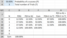
I have several tables that show how to use various probability and statistical functions. Depending on the initial conditions, many of them change not only the results but the number of valid results. This table intended to illustrate the Binom.Dist function is a good example.

It's set up to show the results for a total of 5 trials. But suppose I want to see resutls for 3 trials. If I just change T to 3, I will get a bunch of #NUM errors for those cells with parameters out of range. And the Sum of the P(N) values also fails.

I "solved" this problem by adding IF functions to each equation that test for valid parameters.

The table looks nicer, but the equations do not. And the whole purpose of the sheet was to help me remember how to use this function. My other option was to put everything in a UDF that would check for valid parameters and then either return a value or "". But then the function I am trying to illustrate is even less obvious buried in code.

I looked into custom and conditional formats, but they only change the appearance of the cell. The data would still be an error, which would cause any sums or averages to fail.

Please let me know if there is a better way.

I would post the mini sheet, but I have some unlimited ranges, which causes it to hang.

 

[Alex Blakenburg]

At the moment you are capturing very specific errors and returning "".
If you are happy return "" for all errors you could replace the condition part
=IF(condition,calculation,"")
with
=IFERROR(calculation,"")

 

[JenniferMurphy]

At the moment you are capturing very specific errors and returning "".
If you are happy return "" for all errors you could replace the condition part
=IF(condition,calculation,"")
with
=IFERROR(calculation,"")

Very nice. That has a couple of advantages:

1. It's simpler, so the target formulas are less obscured.
2. It relieves me of the need to figure out what the error conditions are.
3. And that eliminates one source of errors -- me. The values in G11 & H11 were missing in the tables above because I miscoded the error condition as "@N<T". It should have been "@N<=T", proving that Binom.Dist is better at detecting errors than I am.

Here's the improved table with the new values shown in yellow.

I'm going to mark this as solved, because I doubt anyone has a better solution. If they do, I'll change it.

Thanks for the help.

 

[Alex Blakenburg]

That's fine. Thanks for letting me know and glad I could help.

 

[StephenCrump]

Nothing wrong with Alex's solution, but with 365 you could also do:

	A	B	C
1	p	50%
2	T	3
3
4	N	P(N)	etc
5	0	12.5%
6	1	37.5%
7	2	37.5%
8	3	12.5%
9
Sheet1

Cell Formulas
Range	Formula
A5:A8	A5	=N
B5:B8	B5	=BINOM.DIST(N,T,p,)
Dynamic array formulas.

Named Ranges
Name	Refers To	Cells
p	=Sheet1!$B$1	B5
T	=Sheet1!$B$2	A5:B5

where N: =SEQUENCE(T+1,,0)

 

[offthelip]

I use this simple macro add iferror to existing formula:

Sub addiferror()
cform = ActiveCell.Formula
cform2 = Mid(cform, 2)
'cform3 = "=iferror(" & cform2 & ","""")"
cform3 = "=iferror(" & cform2 & ",FALSE)"

 ActiveCell.Formula = cform3
End Sub

You can change it to get FALSE or "" as required

 

[JenniferMurphy]

Nothing wrong with Alex's solution, but with 365 you could also do:

Wow! That looks like it could be powerful. But I'm going to need to study it. I was able to generate an array of values for N. but I couldn't see how you got the P(N) column. I tried naming the Sequence array and using that as an argument, but that didn't work.

Do you know of a good tutorial on this? I checked several YouTube videos, but they are all very primitive. They just show you how to generate various lists.

Thanks

 

[StephenCrump]

I used Name Manager to create a new name N:

Alternatives:

	A	B	C	D
1	p	50%
2	T	3
3
4	N	P(N)	P(N)	P(N)
5	0	12.5%	12.5%	12.5%
6	1	37.5%	37.5%	37.5%
7	2	37.5%	37.5%	37.5%
8	3	12.5%	12.5%	12.5%
Sheet1

Cell Formulas
Range	Formula
A5:A8	A5	=N
B5:B8	B5	=BINOM.DIST(N,T,p,)
C5:C8	C5	=BINOM.DIST(A5#,T,p,)
D5:D8	D5	=BINOM.DIST(AnotherN,T,p,)
Dynamic array formulas.

Named Ranges
Name	Refers To	Cells
AnotherN	=Sheet1!$A$5#	C5:D5
p	=Sheet1!$B$1	B5:D5
T	=Sheet1!$B$2	A5:D5

If you don't mind spending $5, I can recommend the house brand: Excel Dynamic Arrays Straight to the Point 2nd Edition

I'm not an Excel video watcher, but perhaps others can suggest good link(s) for you?

 

[JenniferMurphy]

I use this simple macro add iferror to existing formula:

Sub addiferror()
cform = ActiveCell.Formula
cform2 = Mid(cform, 2)
'cform3 = "=iferror(" & cform2 & ","""")"
cform3 = "=iferror(" & cform2 & ",FALSE)"

 ActiveCell.Formula = cform3
End Sub

You can change it to get FALSE or "" as required

I'll have to study that one, too. Thanks