How to use solver to determine which modules to pass/fail to maximize GPA

[excellol]

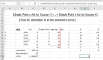
I have the option to grade any module as "s/u" this semester and the modules with "s/u" grading will not be included in GPA calculation.

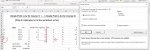
I tried using solver to determine which module to grade as "s/u" in order to maximize my gpa for this sem but results were wrong. I set the objective to maximize C16 (cGPA) and changing variable cells D8:D12. How should i go about setting the constraints?

Is it possible for solver to determine which module to grade as "s/u" and which grade the remaining modules must have in order to maximise my gpa? If so, how do i set up my cells and solver to derive this solution?

Column A is the hardcoded grade and column D has the formula =VLOOKUP(cell from column A,$H$7:$I$14,2,FALSE).
Column E is to calculate the individual elements in the numerator. It has the formula column C * column D
Cells C14 and C15 are just summing up the elements in the numerator and denominator of the formula. You can assume that the formula is correct.

 

[Eric W]

Welcome to the forum!

I'm not so sure I can assume that your C12:C14 formulas are correct. They don't seem to follow the rules I'm familiar with for weighted averages. But follow along and see if this helps. Consider this layout:

Book1
	A	B	C	D	E	F	G	H	I
7		y4s1	AU (weights)	Grade point	wgt avg	use?		A	5
8	a	4013	4	5	20	1		A-	4.5
9	b	3214	2	3.5	7	0		B+	4
10	a	3014	3	5	15	1		B	3.5
11	s	4011	0	0	0	1		B-	3
12	s	2011	0	0	0	1		C+	2.5
13								C	2
14		numerator	355.32			4		s	0
15		denominator	81
16		cGPA	4.386667		cGPA	4.666667
17					cGPA (used)	5
Sheet25

Cell Formulas
Range	Formula
D8:D12	D8	=VLOOKUP(A8,H$7:I$14,2,0)
E8:E12	E8	=C8*D8
F14	F14	=SUM(F8:F12)
F16	F16	=SUM(E8:E12)/SUM(C8:C12)
F17	F17	=SUMPRODUCT(E8:E12,F8:F12)/SUMPRODUCT(C8:C12,F8:F12)

The cGPA formula I used is in F16, the sum of the weighted values divided by the sum of the weights. I then added the F8:F12 column. This is a binary value, 0 or 1, and just means whether you should use that row or not. A 0 would be your s/u row, the rest should be 1. I then created the F17 formula which calculates the weighted average without the 0 column. In the setup shown, the cGPA is 4.6, but if you remove row 9, the cGPA is 5. Removing row 11 or 12 has no effect since the weight is 0.

Given this setup, set up Solver as shown:

That'll spin through all the options and should give you the answer you want. Hopefully you should be able to adapt it to your situation. Good luck!

 

[Eric W]

And just because I like playing with arrays, you can solve this kind of thing with a formula, without Solver. Even though the formula is more complicated than anyone in his right mind would want to maintain.

Book1
	A	B	C	D	E	F	G	H	I
7		y4s1	AU (weights)	Grade point	wgt avg	use?		A	5
8	a	4013	4	5	20	1		A-	4.5
9	b	3214	2	3.5	7	0		B+	4
10	a	3014	3	5	15	1		B	3.5
11	s	4011	0	0	0	1		B-	3
12	s	2011	0	0	0	1		C+	2.5
13								C	2
14		numerator	355.32			4		s	0
15		denominator	81
16		cGPA	4.386667		cGPA	4.666667
17					cGPA (used)	5
18					Row to skip:	2
Sheet25

Cell Formulas
Range	Formula
F18	F18	=MATCH(MAX(MMULT({1,1,1,1,1},(1-MUNIT(5))*E8:E12)/MMULT({1,1,1,1,1},(1-MUNIT(5))*C8:C12)),MMULT({1,1,1,1,1},(1-MUNIT(5))*E8:E12)/MMULT({1,1,1,1,1},(1-MUNIT(5))*C8:C12),0)
Press CTRL+SHIFT+ENTER to enter array formulas surrounded with curly braces.

 

[excellol]

Hi Eric

I'm not so sure I can assume that your C12:C14 formulas are correct. à do you mean C14:C16?

In C14, the formula = total weighted average for the graded courses in past semesters + weighted average of current semester (which is 45 in the attached picture)

In C15, the formula = total graded AUs in past semesters + graded AUs of current semester (which is 9 in the attached picture)

C16 is just C14/C15



The AUs for C11 and C12 are 0 because an IF formula was used: =IF(A12=$H$14,0,3)

This means if the cell in column A = H14, then the AU = 0 as that means s/u was used on that module, thus removing it from the GPA calculation automatically



Why does F14 have the constraint of 4? I can exercise s/u for all modules so should it be <=5?

I copied your set up and ran solver but it didn’t change anything… (ie F17 still showed a value of 5)

 

[Eric W]

========================================================================================
Hi Eric

I'm not so sure I can assume that your C12:C14 formulas are correct. à do you mean C14:C16? Yes, sorry.

In C14, the formula = total weighted average for the graded courses in past semesters + weighted average of current semester (which is 45 in the attached picture)

In C15, the formula = total graded AUs in past semesters + graded AUs of current semester (which is 9 in the attached picture)

C16 is just C14/C15
How do the past semesters GPAs affect the current GPA?


The AUs for C11 and C12 are 0 because an IF formula was used: =IF(A12=$H$14,0,3)

This means if the cell in column A = H14, then the AU = 0 as that means s/u was used on that module, thus removing it from the GPA calculation automatically
I didn't realize that s meant s/u. I assumed it was a failing grade.



Why does F14 have the constraint of 4? I can exercise s/u for all modules so should it be <=5?
I didn't realize that you could exercise s/u for more than one module, so yes you can change the constraint to be <=5.

I copied your set up and ran solver but it didn’t change anything… (ie F17 still showed a value of 5)
The setup I showed had the results after I ran the Solver, so running it again wouldn't change anything.

=====================================================================================================

Given this new information, I'd recommend using the actual grades in A11:12, the actual weights in C11:12, and change the constraint as mentioned. Then once you rerun the Solver, you'll have a set of 1s and 0s in F8:F12 showing which classes to include. If you have more or less than 5 classes, you'll have to change the ranges in the Solver setup.

 

[excellol]

How do the past semesters GPAs affect the current GPA?
its on a cumulative basis. so for each semester, the calculation for the cumulative gpa of previous semesters is added on to the calculation of the current semester's gpa to obtain the new cumulative gpa.

setup 1:
I don't quite get you on how i should setup the data for solver. this is what i've done to set it up before running solver:
1) added column F (use) and inserted a formula =IF(A8=$H$14,0,1) --> if cell in column A is = s, the value will be 0, else its = 1
2) F13 sums up all 0s and 1s
3) i randomly assign a grade to each module
4) in cell H16, i followed your formula of =SUMPRODUCT(E8:E12,F8:F12)/SUMPRODUCT(C8:C12,F8:F12)

5) ran solver with the following parameters

results: for the last module, i originally assigned "s" to A12 and thus F12 was 0 initially. Now it changes to 1 (although this module is not taken into account anyway due to the AU = 0).
1) Is this how it should work?
2) Is it possible for solver to show me the grade i should obtain for each module (as these grades are just guesses) + which module(s) to s/u in order to maximize the gpa for the current semester?

_______________________________________________________
setup 2: everything is the same as above except that i change the objective cell to C16 (cumulative GPA)

results didn't change at all?

sorry for the long post but i really want to know how this works

 

[Eric W]

I think we're talking about the same thing, but in different ways, and that is confusing. Let's first try to clarify some of the math. The cumulative GPA is dependent on the current semester's GPA, true, but if you want to maximize the cumulative GPA you just need to maximize the current semester GPA. You can create a formula to figure out what your new cGPA will be based on your estimated/real GPA for this semester, but you don't want to include the cGPA in the calculations for the current GPA, it'll just make it more complicated and won't change anything.

Next, we can set up the Solver to figure out what grades you should get to maximize the GPA, but it should come as no surprise that it'll tell you to get all A's. You could throw in an additional constraint along the lines of "I have x hours to study, I could study enough to get an A in one class, and a B in another but not both." But again, it would tell you to get the A in the class with the biggest weight. So unless you have some constraints we can quantify in formulas, it's best to let this sit for now.

Also, as I'm thinking about it now, if you're trying to maximize the GPA, and you can exclude any of the classes, it'll look for the class with the highest grade, and then exclude any other classes with a lower grade. The reason is that any lower grade will drag down the average, to a greater or lesser extent depending on the weight.

So this really answers your question without using Solver at all. However, I was in college too, and I was doing these same kind of calculations to try to figure out what I needed. The difference is that I was using a target value. To graduate with some honors, I needed a cumulative GPA of at least 3.7 (on a scale to 4). So I would work out what I needed to maintain that score. And maybe that's why you included the cGPA. But you can't just say "maximize" or it'll say "all A's".

In looking at your original layout, I think I now see what you were trying to do. You wanted to vary the grades in A8:A12 and figure out the effect on the GPA and cGPA. And looks like it was pretty much there. With your C8:C12 formulas, the GPA would just be SUMPRODUCT(C8:C12,D8:D12)/SUM(C8:C12), and I'll assume your cGPA formula would be correct too. The problem is varying the grades in A8:A12, since the Solver works in numbers, not letters. We could solve that problem by adding another column (like my use? column in column F) that is allowed to vary from 1 to 8, and then the A8 formula is =CHOOSE(F8,"A","A-","B+","B","B-","C+","C","S"). And then another formula in F14 that sums up the values from F8:F12. And then we'd have everything we'd need to run the Solver, although the question would be slightly different than you originally proposed. It would go something like: Minimize F14 (what are the lowest grades I can get), with the constraints that F8:F12 are >=1 and <=8 (valid grades), and that C16 is greater than 4.3.

Kinda long-winded, but I hope it helps! Let me know.

 

[excellol]

In looking at your original layout, I think I now see what you were trying to do. You wanted to vary the grades in A8:A12 and figure out the effect on the GPA and cGPA. And looks like it was pretty much there. With your C8:C12 formulas, the GPA would just be SUMPRODUCT(C8:C12,D8:D12)/SUM(C8:C12), and I'll assume your cGPA formula would be correct too. The problem is varying the grades in A8:A12, since the Solver works in numbers, not letters. We could solve that problem by adding another column (like my use? column in column F) that is allowed to vary from 1 to 8, and then the A8 formula is =CHOOSE(F8,"A","A-","B+","B","B-","C+","C","S"). And then another formula in F14 that sums up the values from F8:F12. And then we'd have everything we'd need to run the Solver, although the question would be slightly different than you originally proposed. It would go something like: Minimize F14 (what are the lowest grades I can get), with the constraints that F8:F12 are >=1 and <=8 (valid grades), and that C16 is greater than 4.3.

Kinda long-winded, but I hope it helps! Let me know.

lol minimizing F14 resulted in solver telling that I should get A for all subjects, which is impossible.

Never I'll just do the manual way and change the grade for each to see how the GPA changes. Thanks for the help Eric

 

[Eric W]

After I wrote post 7, I realized I got the formula backwards. Instead of

=CHOOSE(F8,"A","A-","B+","B","B-","C+","C","S")

it should be

=CHOOSE(F8,"S","C","C+","B-","B","B+","A-","A")

which would explain the result you got. You can give that a shot, or do a little experimentation manually like you said. Sorry we didn't get it all working ideally! It's an example of how working remotely can be tough. Hope you get it sorted.