Hyperlink with Index Formula - "Cannot Open Specified File"

[norts55]

Hello,
I have searched to find a solution to this and it seems there may be many out there but I have tried many and nothing works for me. I am at a total loss.

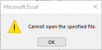
I am trying to create a hyperlink with the index formula. -See below. Every time I click in the cell I get a message box stating "Cannot Open Specified File"

Can someone please help with this?

=HYPERLINK(INDEX('DOT Avg Prices'!$G$2:$G$3000,MATCH(F649,'DOT Avg Prices'!$B$2:$B$3000,0)),VLOOKUP(F649,'DOT Avg Prices'!$B$2:$G$3000,6))

 

[GraH]

Hi,

What is index returning and what is the hyperlink you expect to get? Can you upload some sample data using tbe XL2BB add-on please.

 

[norts55]

Hello,
Thank you for the response. I have a table on sheet DOT Avg Prices. The index will use the contents of cell F649 and column B on sheet DOT Avg Prices to find a match and then use what is in column G from the sheet DOT Avg Prices. - I hope I explained that correctly.

 

[GraH]

Hi, I understand the formula and I know it can be difficult to explain, hence showing some data might help.
You did not exactly answer what the hyperlink is supposed to do: link to a site, a cell reference on a sheet (what I suspect you are after), another workbook,...

Perhaps explain what do you want to accomplish.

 

[norts55]

Thank you for hanging in there with me.

What I need the hyperlink to do, is link to the cell the index finds. It is in the same workbook but a different sheet. The sheet name is 'DOT Avg Prices'.

 

[GraH]

Please try
=HYPERLINK("#'DOT Avg Prices'!G"&MATCH(F649,'DOT Avg Prices'!$B$2:$B$3000,0)+1,VLOOKUP(F649,'DOT Avg Prices'!$B$2:$G$3000,6) )

 

[Fluff]

Another option
=HYPERLINK("#"&ADDRESS(MATCH(F649,'DOT Avg Prices'!$B$1:$B$3000,0),7,,,"DOT Avg Prices"),VLOOKUP(F649,'DOT Avg Prices'!$B$2:$G$3000,6,0))

The only real difference is the Vlookup is looking for an approximate, adding the last 0 makes it an exact match. Whether you need that depends on your data.

 

[norts55]

Both of these work wonderfully! Thank you both very much!

 

[Fluff]

Glad we could help & thanks for the feedback.