I want to conditionally format a cell if two other cells return no value

[Tristram_ZX81]

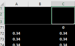
In below picture, C column is sum of A:B. However, I want the C column to go red if there is no value in either A or B, as in row 280, 284, 285 and 288 below. However, I can only find how to conditionally format 'blank' cells. The problem is, these cells aren't blank, they have IF formula in them referring to the data in columns D onwards. So I want C to flag red if the IF formula returns no data for either column. Sometimes the A and B (and C) will return a 0 (zero); I don't want this to trigger the conditional formatting. Any ideas?

 

[steve the fish]

How about:

=AND(A1="",B1="")

or

=OR(A1="",B1="")

whether you want both or either.

 

[Tristram_ZX81]

Thanks for the reply Steve. Sadly, these haven't worked. In image below only row 13, 19 and 27 should be red below as everything else has a 0 figure or higher in it.

 

[steve the fish]

Looks like you need to use the AND not the OR

 

[Tristram_ZX81]

Sorry Steve that's not quite working either

 

[steve the fish]

Tell me exactly what the CF formula says and what its applied to. Its impossible for what i gave you to format like that. Is there other CF on those cells?

 

[Tristram_ZX81]

Thanks Steve. Cell A4 is

= IF(ISNUMBER(SEARCH("football",Q4)),0.1, IF(ISNUMBER(SEARCH("rugby",Q4)),0.1, IF(ISNUMBER(SEARCH("tennis",K4)),0, IF(ISNUMBER(SEARCH("quidditch",K4)),1, IF(ISNUMBER(SEARCH("golf",K4)),1, IF(ISNUMBER(SEARCH("nfl",K4)),0.5,""))))))


Cell B4 is the same but with different sports. (The above is a simplified version, there's actually 64 IF conditions in the actual formula).

Cell C4 is =IF(OR(A4=0.1,B4=0.1),0.1,IF(OR(A4>=0.2,B4>=0.2),SUM(A4:B4),""))

 

[steve the fish]

Its not the formulas in the cells i would need. Its the conditional formatting formula you are using and what its applied to. The formula i gave you is to be used for conditional formatting.

 

[Tristram_ZX81]

Ah. The only conditional formatting I've used is the codes you gave me, I tried

=AND(A1="",B1="")

and then

=OR(A1="",B1="")

The above screen shots are the results of using conditional formatting formula.

 

[steve the fish]

Applied to?