IF, but IF

[qwzky]

Hi! I am having a hard time figuring this out.
Maybe this is also about IFS function. My guess is that maybe it is also about COUNTIF.
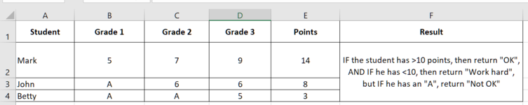
Simply put, my problem looks like this:

I tried

=IFS(E2>10;"OK";IF(E2<10;"Work hard";"WORK HARD"); COUNTIF(B2:D2;"A"))

Please, help me with that. I really need that for my school as a principal.

 

[Eric W]

Welcome to the MrExcel forum!

Try:

Book1
	A	B	C	D	E	F
1	Student	Grade 1	Grade 2	Grade 3	Points	Result
2	Mark	5	7	9	14	OK
3	John	A	6	6	8	Not OK
4	Betty	A	A	5	3	Not OK
Sheet5

Cell Formulas
Range	Formula
F2:F4	F2	=IF(COUNTIF(B2:D2,"A"),"Not OK",IF(E2>10,"OK","Work hard"))

It looks like your version of Excel uses semi-colons instead of commas in the formula, make sure to change those when you enter it.

 

[qwzky]

Oh my, thank you I am so happy for this. Can you also please tell me what to do if I want to introduce multiple IFS in the green section?
For instance,

=IF(COUNTIF(B2:D2,"A"),"Not OK",[B][COLOR=rgb(65, 168, 95)]IF(E2>10,"OK","Work hard")) and/but if E2<5,"5",""[/COLOR][/B]

 

[qwzky]

I mean here:

=IF(COUNTIF(B2:D2,"A"),"Not OK",IF(E2>10,"OK","Work hard")) and/but if E2<5,"5",""

 

[Alex Blakenburg]

When did you want it to be "" ?

=IF(COUNTIF(B2:D2,"A"),"Not OK",IF(E2>10,"OK",IF(E2>=5,"Work hard","5")))

I often use this layout you find it helps

=IF(COUNTIF(B2:D2,"A"),"Not OK",
    IF(E2>10,"OK",
        IF(E2>=5,"Work hard",
            "5")))

Alt+Enter gives you the new line and then just spaces for indenting

 

[qwzky]

With your help, I managed to come up with the solution:

=IF(COUNTIF(C6:E6;"A");"";IF(F6<=9;"10";IF(F6<=19;"9";IF(F6<29;"8";IF(F6<=39;"7";IF(F6<=49;"6";IF(F6<=59;"5";IF(F6<=69;"4";IF(F6<=79;"3";IF(F6<=89;"2";IF(F6<=300;"1";"")))))))))))

I understood that the FALSE is actually another IF (see below):

SC-uri automate REDONE.xlsm
	C	D	E	F	G	H
2	Grade 1	Grade 2	Grade 3	Points	Result
3	5	7	9	14		9
4	A	6	6	8
5	A	A	5	3
6	5	6	5	55		5
Sheet2

Cell Formulas
Range	Formula
H3:H6	H3	=IF(COUNTIF(C3:E3,"A"),"",IF(F3<=9,"10",IF(F3<=19,"9",IF(F3<29,"8",IF(F3<=39,"7",IF(F3<=49,"6",IF(F3<=59,"5",IF(F3<=69,"4",IF(F3<=79,"3",IF(F3<=89,"2",IF(F3<=300,"1","")))))))))))

 

[Alex Blakenburg]

At some point you might want to consider moving to using a lookup table.
The table can go anywhere in the workbook but the current vlookup formula needs it to be called tblGradeGrp.

Also I don't know if you realise it but your current If statement is returning the numbers as text by wrapping them in quote marks.
This means you can't use and arithmetic formulas on them eg you have "10" it is likely you just need 10.

20210723 Vlookup Grouping.xlsx
	A	B	C	D	E	F	G
1
2			Grade 1	Grade 2	Grade 3	Points	Result
3			5	7	9	14	9
4			A	6	6	8
5			A	A	5	3
6			5	6	5	55	5
7
8
9
10
11
12	Grade Grouping
13	Enter To column in ascending order
14	TableName	tblGradeGrp
15
16
17	Calc	Input	Input
18
19	From	To	Result
20	0	9	10
21	10	19	9
22	20	29	8
23	30	39	7
24	40	49	6
25	50	59	5
26	60	69	4
27	70	79	3
28	80	89	2
29	90	300	1
Sheet2

Cell Formulas
Range	Formula
G3:G6	G3	=IF(COUNTIF(C3:E3,"A"),"",VLOOKUP(F3,tblGradeGrp,3,TRUE))
A20:A29	A20	=IF(B19="To",0,N(B19)+1)

 

[Eric W]

I'm glad you got it worked out. Sometimes you can use one of the lookup functions to shorten the formula, like so:

Book1
	C	D	E	F	G
2	Grade 1	Grade 2	Grade 3	Points	Result
3	5	7	9	14	9
4	A	6	6	8
5	A	A	5	3
6	5	6	5	55	5
Sheet3

Cell Formulas
Range	Formula
G3:G6	G3	=IF(COUNTIF(C3:E3,"A"),"",LOOKUP(F3,{0,10,20,30,40,50,60,70,80,90,301},{10,9,8,7,6,5,4,3,2,1,""}))

It looks like Alex beat me to the punch. His formula uses an external table (arguably better), and my formula has it embedded within the formula.

 

[qwzky]

I'm glad you got it worked out. Sometimes you can use one of the lookup functions to shorten the formula, like so:

Book1
	C	D	E	F	G
2	Grade 1	Grade 2	Grade 3	Points	Result
3	5	7	9	14	9
4	A	6	6	8
5	A	A	5	3
6	5	6	5	55	5
Sheet3

Cell Formulas
Range	Formula
G3:G6	G3	=IF(COUNTIF(C3:E3,"A"),"",LOOKUP(F3,{0,10,20,30,40,50,60,70,80,90,301},{10,9,8,7,6,5,4,3,2,1,""}))

It looks like Alex beat me to the punch. His formula uses an external table (arguably better), and my formula has it embedded within the formula.

This formula doesn't seem to exclude the rows containing „A”. I tried to work around cell formatting as number, but it still doesn't work. You were right about it: I would like to use those results in calculating average. Can you think of a way to do modify the formula that I posted as a final solution?

 

[Alex Blakenburg]

I am not sure Eric would still be online it is quite late where he is. I am in Australia.

This formula doesn't seem to exclude the rows containing „A”.

Eric's formula has exactly the same exclusion code as yours and I can confirm that it definitely returns "" if any of the Grades on that line have an "A" in them. ie =IF(COUNTIF(C3:E3,"A"),""

I tried to work around cell formatting as number, but it still doesn't work. You were right about it: I would like to use those results in calculating average. Can you think of a way to do modify the formula that I posted as a final solution?

As I pointed out earlier if you wanted to stick with your formula but have the results return numbers so you can work with them, all you need to do is remove the quote marks "" that you have around the numbers.
I have done that below.

    =IF(COUNTIF(C3:E3,"A"),"",IF(F3<=9,10,IF(F3<=19,9,IF(F3<29,8,IF(F3<=39,7,IF(F3<=49,6,IF(F3<=59,5,IF(F3<=69,4,IF(F3<=79,3,IF(F3<=89,2,IF(F3<=300,1,"")))))))))))