If Cell = " " Then... populate a specific cell on another worksheet

[kbishop94]

I'm probably pushing my luck with the # of questions I'm throwing at you guys today, but I'm stuck again (its another 'simple' problem, but unfortunately those are the ones that tend to stump me )

Here is what I am attempting to do:

the range on this worksheet ("HELPER1") needs to be A1:A6

Column A can have UP TO 6 results.

The data will always be formatted the same, and can include the following names (in any order too):

"Rosenberg"
"El Campo"
"Site 239"
"529 Warehouse"
"Technology Center"
"Other"

they will be sorted by the number that is associated with the particular name that is located in column B.

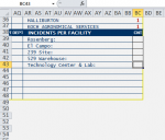
On another worksheet "STATISTICS", I have the same names that can be found in column A on "HELPER1" in the following rows and columns: The names on this worksheet will always be static (so the string "Rosenberg" will always be in cell AR:39 on this worksheet.)

on "STATISTICS" worksheet, these are the static positions for each name's value (which is to be the number of occurrences shown on the "HELPER1" sheet):
the number for each needs to be:
"Rosenberg" = "BC39"
"El Campo" = "BC40"
"239 Site" = "BC41"
"529 Warehouse" = "BC42"
"Technology Center & Lab" = "BC43"
"Other" = "BC44"

I have the default value set to ZERO. If one of the possible names does have an occurrence on "HELPER1" then the new value will be copied over the '0' that is in that cell (otherwise, if it doesn't, then it will telling the user: "Rosenberg has 0 incidents")


Although Column A can have up to 6 possible names on the "HELPER1" sheet, at times it may only have one (but it will never be empty.) Each name will only occur one time in column A as well.

What i've been trying to make work for my code basically says this (I'll use one of the strings "Rosenberg" as an example in my crude description below):

If, any of the cells in the range A1:A6 (on HELPER1), equal "Rosenberg", then copy the number in the column beside the Rosenberg row (which is going to be '18' in column B) and then paste it to the specific cell for that 'If' possibility, which for Rosenberg is going to be in "BC:39" on the sheet "STATISTICS". Repeat for each of the other 5 possibilities for the other names.

Sorry for all the questions, but I just about got this finished!

 

[kennypete]

Here you go; in the example below I have two Sheets, Sheet1 and Sheet2. Your 6x2 named range is in Sheet1. This is Sheet2:

Book1
	AP	AQ	AR	AS
38	CNT	DEPT	INCIDENTS PER FACILITY	CNT
39			Rosenberg	18
40			El Campo	7
41			Site 239	2
42			529 Warehouse	1
43			Technology Center & Lab	0
Sheet2

Cell Formulas
Range	Formula
AS39:AS43	AS39	=IFERROR(VLOOKUP(AR39,HELPER1,2,FALSE),0)

i.e. Cells AS39- are identical but for the incremental reference to the ARxx cell.

The following illustrates this updating as Sheet1 is updated:

 

[kbishop94]

Here you go; in the example below I have two Sheets, Sheet1 and Sheet2. Your 6x2 named range is in Sheet1. This is Sheet2:

Book1
	AP	AQ	AR	AS
38	CNT	DEPT	INCIDENTS PER FACILITY	CNT
39			Rosenberg	18
40			El Campo	7
41			Site 239	2
42			529 Warehouse	1
43			Technology Center & Lab	0
Sheet2

Cell Formulas
Range	Formula
AS39:AS43	AS39	=IFERROR(VLOOKUP(AR39,HELPER1,2,FALSE),0)

i.e. Cells AS39- are identical but for the incremental reference to the ARxx cell.

The following illustrates this updating as Sheet1 is updated:
View attachment 5865

Wow, that is really cool.

THANK YOU!

 

[kennypete]

All good @kbishop94, you’re welcome. Just bear in mind the entries need to be identical: e.g. in your source you have Site 239 and 239 Site. Even extra spaces in the source will cause you trouble. Cheers