If-then Calculation Across Rows/Columns Based On Other Columns.

[AutoMike]

Greetings guru's, total excel Newbie here. So new, I don't even know how to properly term what I'm trying to do in order to search it. I'm confident there's some excel calculation guru's here who can explain it to me like I'm 5 months old (in excel years), hopefully I can explain the question/want adequately. See the attached Image. I'm a project manager, I assign tasks, and track work load to predict lead times, follow performance, balance jobs etc. I've managed to use basic google searches to make excel a pretty powerful work calendar for me. On various tabs I know how much I need to manufacture with how much lead time, how many base units are prepared to fulfill those orders, how much I've made of each product type year to date by production days with holidays subtracted and so on. All in all, it's the clearest view of our actual productivity my company has ever had and certainly the least labor intensive view.

I've google poke and played through all those calculations and gotten them working. But I'm stuck on a calculation I want that I can't even figure out how to properly search.
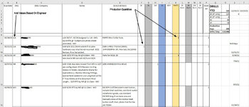
In the attached image, in column B, I assign jobs to specific people/groups. In columns F - K there are specific components of those jobs represented as values. So in the attached example, JLA is assigned a parts job, and a single 2K job (that 2K value could be 1, 2, 3, 4, 5 or more and represents a total number of drill units). Over the course of a year, I want to track JLA's performance and productivity to provide feedback and to inform my assignment decisions to balance work-load and skill development in new areas. In the pending calendar I want to track his pending work load by the same method.
In a nutshell I want to create a series of formulas that will say If Column B value is JLA on a particular row, then Count the SUM of the Column F According to ALL the rows where JLA is assigned. I already have a calculation that tells me the YTD for column F is 119 for ALL engineers in R2, but I also want the sub value for each individual engineer for each of job types F (and G-K)
In the tiny example shown, I'd expect the value for JLA to be 1 for 2K, and 0 for 5K, but if the value in F10 were 5, I'd expect that sum to be 5. I ran across calculations that would basically tell me how many times JLA occurred with ANY value in F, but not that would add up the sum of values. In this example, where NR is the value in B, I'd expect his 2K sum to be 0, his 5K sum to be 1, etc.

 

[RobP]

Hi,

I think the formula you are looking for would be thus:

=SUMIF(B:B,"JLA",F:F)

which essentially says Sum the Column F for the Rows in B that contain JLA. You should be able to modify it for your other columns easily I think ?

cheers
Rob

 

[RobP]

Or, if you prefer to put "JLA" into a cell, for example I typed it into A1 here, you could just use this to total whichever operator you typed into cell A1, leaving it flexible for you to check any operator you wanted just by entering his initials.

=SUMIF(B:B,A1,F:F)

 

[AutoMike]

Hi,

I think the formula you are looking for would be thus:

=SUMIF(B:B,"JLA",F:F)

which essentially says Sum the Column F for the Rows in B that contain JLA. You should be able to modify it for your other columns easily I think ?

cheers
Rob

Excellent Rob! Thanks, So could I modify this to "=SUMIF(B:B,"JLA",F:K)" in order to get all of the items to all of the categories where JLA is the value in column B?

 

[RobP]

Ah, my apologies - I hadn't clocked you wanted to total all the columns in one hit.

OK, so slight modification, try this one :

=SUM((F4:K8)*(--(B4:B8=A1)))

where again, I assume your operators are in ColB, and your data is in F:K. For this one, you have to specify totally your data range (ie. from row x to row Y - which in my case was rows 4 to 8 for example..)

 

[AutoMike]

Ah, my apologies - I hadn't clocked you wanted to total all the columns in one hit.

OK, so slight modification, try this one :

=SUM((F4:K8)*(--(B4:B8=A1)))

where again, I assume your operators are in ColB, and your data is in F:K. For this one, you have to specify totally your data range (ie. from row x to row Y - which in my case was rows 4 to 8 for example..)

You didn't miss my question in the post at all, your answer worked so well I got excited about playing with the formula to work out other aspects of the data! .. This new formula lost me a little, going to have to study this later to learn to read it properly and then translate it. In this part "(F4:K8)*(--(B4:B8=A1)" I'm expecting I actually need (F:K)*(--B:B=A1) because I'm inserting new rows with new jobs all year, but I'm not clear why the multiplication between "(F4:K8)" and "(--(B4:B8=A1)" and why the two minus signs in "(--(B4:B8=A1)" are there (sorry I wasn't exaggerating when I said explain it like I'm 5 months old in excel years and when I described my method thus far as "poke and play" google searching for calculations.)

 

[RobP]

well, its unfortunate that when having multiple columns, you need to specify the data range (rather than just the columns) - I think mainly due to the way the array formula works. There's always a thousand ways to do things, and so to try and explain it a little easier, this formula will also do the same thing:

=SUMPRODUCT((B2:B9=A1)*(F2:K9))

The first expression inside SUMPRODUCT is the criteria, which gives you an array of TRUE or FALSE values if it finds the correct initials in the row. So it looks like this:

{TRUE;TRUE;FALSE;FALSE;TRUE;FALSE;FALSE;FALSE} (where TRUE = JLA found. TRUE takes the value of 1, FALSE takes the value of 0 in Excel formulas.)

This (effective array of 1's and 0's) is then multiplied in order by the values in the data range F2:K9. F2:K9 looks like this to the formula:

{1;2;1;1;1;2;2;2;1;1;2;2} eg. starts top left of your range, finishes bottom right, numbers placed in order)

So the actual result inside SUMPRODUCT is thus:

{1;2;1;0;0;0;0;2;0;0;0}

so when it SUMS those up (now that its done the PRODUCT (or multiplication) part .. it returns a 6.

In my previous formula, in the same way it basically SUMS the PRODUCT of two results in the same way. The "--" you see in it is telling that part to return an array of TRUE/FALSE values..

Hope its clear. If you are "inserting" rows into your data, generally the formula will update itself. whereas if you just add a row on the bottom, it won't.

 

[AutoMike]

View attachment 77162
well, its unfortunate that when having multiple columns, you need to specify the data range (rather than just the columns) - I think mainly due to the way the array formula works. There's always a thousand ways to do things, and so to try and explain it a little easier, this formula will also do the same thing:

=SUMPRODUCT((B2:B9=A1)*(F2:K9))

The first expression inside SUMPRODUCT is the criteria, which gives you an array of TRUE or FALSE values if it finds the correct initials in the row. So it looks like this:

{TRUE;TRUE;FALSE;FALSE;TRUE;FALSE;FALSE;FALSE} (where TRUE = JLA found. TRUE takes the value of 1, FALSE takes the value of 0 in Excel formulas.)

This (effective array of 1's and 0's) is then multiplied in order by the values in the data range F2:K9. F2:K9 looks like this to the formula:

{1;2;1;1;1;2;2;2;1;1;2;2} eg. starts top left of your range, finishes bottom right, numbers placed in order)

So the actual result inside SUMPRODUCT is thus:

{1;2;1;0;0;0;0;2;0;0;0}

so when it SUMS those up (now that its done the PRODUCT (or multiplication) part .. it returns a 6.

In my previous formula, in the same way it basically SUMS the PRODUCT of two results in the same way. The "--" you see in it is telling that part to return an array of TRUE/FALSE values..

Hope its clear. If you are "inserting" rows into your data, generally the formula will update itself. whereas if you just add a row on the bottom, it won't.

That was pretty epic Rob! I'm pretty sure I followed 90% of that immediately, which is a pretty good pre-coffee return. A second read got me a little further and I'm going to play around with this in my sheet. If I'm following, the multiplication works because the sum product is always based on a value of "1" because JLA only occurs once per row. I appreciate the help! I always insert rows rather than adding at the bottom for the auto correcting formula reason. Some of my calculations still have to be manually updated each time but that is because they have both fixed and moving references (and probably because I lack the knowledge base to develop smarter formulas)
Historically, we've been using 3 (or more) separate calendars to track the work in my company for years and years. I'm very confident that if I spend a couple more hours of time and energy in excel that I'll be able to make a single document that lets us keep better track of ongoing data, accumulate data, and sort priorities better and faster and with less repetition than we ever have in the past. Your first answer gave me results in 5 minutes that in the past would have involved dozens of hours of going through job folders and tabulating results, or else going through a google calendar one event at a time tabulating with a margin of error around 15% or more. We've never had an individual worker productivity result. Your formula added to my sheet plan put hard data in seconds on the 'felt' sense of who is doing what in terms of productivity. Exactly the help I was hoping to find here!

 

[RobP]

Great, glad to have been assistance for you..

cheers
Rob