IFERROR returns zero but that 0 doesn't work with conditional formatting

[nathp]

Firstly please excuse me if this is a stupid questions as I relatively inexperienced with excel.

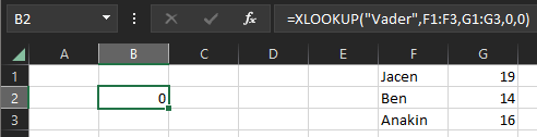
I have an IFERROR formula that preceeds an xlookup. This is set to return a value from the xlookup and a 0 if no value is present in the lookup. I then want to format this cell (along with others) conditionally so that 0 values turn green, 1-2 turns yellow etc). The conditional formatting works perfectly if there is a zero found in the xlookup (or any other number) but when a zero is returned by the iferror then that zero acts as a high number. For instance formatting the returned 0 as a greater than 10 value colours the 0 cell.

Sorry for the bad explanation but any help would be much appreciated.

Thanks

 

[Fluff]

Hi & welcome to MrExcel.
What is the formula you are using?

 

[Jeffrey Mahoney]

Well, have it return a null ("" two quotes) or something else

 

[nathp]

Hi & welcome to MrExcel.
What is the formula you are using?

Thanks for the welcome.
This is the formula
=IFERROR(XLOOKUP("S23P2_ELD1",Alarms!$A$19:$A$43,Alarms!$B$19:$B$43),"0")

 

[Fluff]

You need to remove the quotes from the "0" other wise it's text & not a number.

 

[Wookiee]

Can you please share your formula? Because, depending on how the IFERROR is employed, it might not be necessary because the XLOOKUP function has a parameter to specify what to display if no match is found on the lookup range.

In my example formula below, the second zero represents what to return if there is no match.

=XLOOKUP("Vader",F1:F3,G1:G3,0,0)

 

[nathp]

Well, have it return a null ("" two quotes) or something else

I tried this also but then the blank cell also follows the same (incorrect) conditional formatting when a greater than format is used.

 

[nathp]

Can you please share your formula? Because, depending on how the IFERROR is employed, it might not be necessary because the XLOOKUP function has a parameter to specify what to display if no match is found on the lookup range.

In my example formula below, the second zero represents what to return if there is no match.

=XLOOKUP("Vader",F1:F3,G1:G3,0,0)

This is sounding positive. To be honest, someone else created the xlookup as I had no idea how to do it

 

[AhoyNC]

There is an argument in the XLOOKUP for "if not found".
Try changing your formula to something like the example below.
Also how did you put the 0 into the IFERROOR. Did you put quotes around it "0" which would make text and not numeric.

Book1
	A	B	C	D	E
1	n	0		a	1
2				b	2
3				c	3
4				d	4
Sheet1

Cell Formulas
Range	Formula
B1	B1	=XLOOKUP(A1,D1:D4,E1:E4,0)

 

[nathp]

You need to remove the quotes from the "0" other wise it's text & not a number.

Perfect - that sorted it. I knew it had to be something simple.
Thank you very much