IFS, rounding and absolute values

[N0t Y0urs]

I am not sure if I am over complicating this or not.

I have the following set up and while excel is great and accurate I need to figure out how to achieve the result I want.

So I have this formula in my size column - =IFS(B13="Aj",(((G12*C13))/$C$3)*$H$4,B13="an",(((G12*B13))/$C$3)*$H$5,B13="au",(((G12*C13))/$C$3)*$F$6,B13="achf",(((G12*C13))/$C$3)*$F$5,B13="acad",(((G12*C13))/$C$3)*$F$4,B13="chfj",(((G12*C13))/$C$3)*$H$4,B13="cadj",(((G12*C13))/$C$3)*$H$4,B13="ea",(((G12*C13))/$C$3)*$H$3,B13="echf",(((G12*C13))/$C$3)*$F$5,B13="ecad",(((G12*C13))/$C$3)*$F$4,B13="eg",(((G12*C13))/$C$3)*$H$3,B13="eu",(((G12*C13))/$C$3)*$F$6,B13="en",(((G12*C13))/$C$3)*$H$5,B13="ga",(((G12*C13))/$C$3)*$H$3,B13="gcad",(((G12*C13))/$C$3)*$F$4,B13="gchf",(((G12*C13))/$C$3)*$F$5,B13="gj",(((G12*C13))/$C$3)*$H$4,B13="gn",(((G12*C13))/$C$3)*$H$5,B13="gu",(((G12*C13))/$C$3)*$F$6,B13="nj",(((G12*C13))/$C$3)*$H$4,B13="nchf",(((G12*C13))/$C$3)*$F$5,B13="ncad",(((G12*C13))/$C$3)*$F$4,B13="nu",(((G12*C13))/$C$3)*$F$6,B13="uj",(((G12*C13))/$C$3)*$H$4,B13="uchf",(((G12*C13))/$C$3)*$F$5,B13="ucad",(((G12*C13))/$C$3)*$F$4,B13="xau",(((G12*C13))/$C$3)*$H$6,B13="xag",(((G12*C13))/$C$3)*$J$3,B13="aus",(((G12*C13))/$C$3)*$F$4,B13="nas",(((G12*C13))/$C$3)*$J$5,B13="nikkei",(((G12*C13))/$C$3)*$J$6,B13="ftse",(((G12*C13))/$C$3)*$L$3,B13="us2000",(((G12*C13))/$C$3)*$L$4,B13="dow",(((G12*C13))/$C$3)*$L$5,B13="s&p",(((G12*C13))/$C$3)*$L$6,B13="dxy",(((G12*C13))/$C$3)*$N$3) and it works but just shudder when I look at it so if it could be more efficient let me know please.

From there I use it to calculate my results. But this is where I get stuck. If I take row 13 for example my size reports as 0.06 I would like to make sure that it an absolute value because this impacts me further into my other calculations. In my results I need to create a formula that does the following:

It looks at B13 (Asset) so it knows what $ value to use. The simple instruction is this (in absolute numbers versus what excel reports)

((((D13*C8)*C4*10*H6)+((D13*C8)*C5*10*H6)+((D13*C6*10*H6)-((D13*C8)*C4*10*H6)+((D13*C8)*C5*10*H6)) = his gives the result of $24.97 however the result should actually be $20.93

So to explain what I am trying to do is use excel to forecast. I want the formula to do something like this:

Results = 10% of size x 12.5 (TP1) x 10 x XAU (Asset identifier B13 = Asset value of H6) + 10% of size x 18.5 (TP1) x 10 x XAU (Asset identifier B13 = Asset value of H6) + 80% of size x 32.5 (TP1) x 10 x XAU (Asset identifier B13 = Asset value of H6) + 0% of size x 225 (TP1) x 10 x XAU (Asset identifier B13 = Asset value of H6)

So based on a size of 0.06 it would be:
0.01 x 12.5 x 10 x 1.30 + 0.01 x 18.5 x 10 x 1.30 + 0.04 x 32.5 x 10 x 1.30 + 0 x 225 x 10 x 1.30

Hope that makes sense as I have spent the weekend reading experimenting with IFERRORS, IFS, ROUNDS and ABSOLUTEs and still stuck

Thanks in advance

 

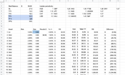[StephenCrump]

Am I asking to much?

.. or too little?

Do you mean? =MIN(250,ROUNDUP(A1,2))

 

[N0t Y0urs]

Let me try it and see what the results will be. Basically to explain what the results of the whole spreadsheet is.

I am using this to forecast the record the actual day trades. So the size is the size of the trade and you start at micro lots being 0.01 from there you can trade up to a maximum of 10,000 but that’s outside my comfort level so my max is set at 250. This section in the first few steps before I get into actúalas and comparisons to analysis the trade. Therefore I’m really wanting to simplify this sheet as much as possible

Hope that makes sense

Also if you look at the inputs sheet that has a guide to what I am wanting without all the bells and whistles

 

[StephenCrump]

If you get stuck, we'll be happy to help with specific questions.

If the questions don't relate to what's been discussed above, you'll be better off starting a new thread.

 

[N0t Y0urs]

If you get stuck, we'll be happy to help with specific questions.

If the questions don't relate to what's been discussed above, you'll be better off starting a new thread.

I’m about to sit on the computer and give it a shot.

I would love to learn more but get caught up so I’m just going one step at a time and try and pull your answers apart so I learn what you’ve done to achieve my result

 

[N0t Y0urs]

So I have edited the formulas to the simplified ones you suggested but I am confused on two aspects.

Here’s my new spreadsheet

Learning excel

Sample A,50,AD,BX,CJ, $ 1.00 B,30,AE,CL,CK, $ 1.51 C,30,AF,CJ,CL, $ 1.77 D,60,AD,BR,BR, $ 1.11 E,90,AE,BU,BU, $ 1.46 F,180,AF,BV,BV, $ 1.10 G,10%,AG,BW,BW, $ 1.41 H,10%,AH,BX,BX, $ 1.41 I,80%,AI,BY,BY, $ 1.41 J,0%,AJ,BZ,BZ, $ 1.41 Comparison ,AK,CA,CA, $ 1.00 #,K,L,M, N ,O, P ,M, N , P

docs.google.com

Where I am confused is the rounding up that should be used in column F and Column E is where I have the maximum value of 250

While the data is not aligned if I look E17 I use 0.09 but my result shows $97 when my result should be $101.52 (K18).
I can’t figure out when in the formula the roundup needs to sit and where the max 250 needs to sit in column E formulas

 

[N0t Y0urs]

I played around further and realised what you meant by the min and that’s now correct so what I have left is the complicated rounding issue

 

[StephenCrump]

In Sample!E16, you have: =MIN($D$12, 250,(H15*$D16)/$D$3*VLOOKUP(VLOOKUP(C16,$P$2:$Q$45,2,), $R$2:$S$21,2,))
with a result of 0.03611.

But $D$12 is 250, so assuming this is the correct cell to determine the maximum value, you can remove the hard-coded 250 from the formula.

And if you want the value to be rounded up to the next whole %, i.e. to 0.04, you'll need:

=MIN($D$12,ROUNDUP(H15*$D16/$D$3*VLOOKUP(VLOOKUP(C16,$P$2:$Q$45,2,),$R$2:$S$21,2,),2))

 

[N0t Y0urs]

Bye George I think we have this solved. Thank you so much. Now on to the next task but thank you

 

[StephenCrump]

Bye George I think we have this solved. Thank you so much. Now on to the next task but thank you

No problem at all. I'm glad you got it working.