Ignore blank rows when charting

[strasbdj]

I have a massive data table that only has data entered into certain columns for each row. I'm trying to create a chart where all of my data is evenly spaced, but because each column has blanks interspersed I get gaps in my chart. How do I get Excel to ignore these and plot the values in a consecutive fashion?

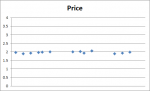
Here is what my chart looks like.

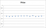
Here is what I want my chart to look like.

I have a feeling there's a very easy solution but my extensive Google searches only tell me how to connect the dots.
Thank you,
Dusty

 

[strasbdj]

Here's an example of the data I'm working with. I made the second chart by removing all the blank rows but I can't do this with the real data because those blank rows correspond to actual values in other columns.

 

[FryGirl]

One easy way, make a pivot chart. Of course, depending on the version of Excel you have which your profile does not say.

Row Labels >> Run #
Values >> Sum of Result

 

[strasbdj]

I'm using Excel 2010. Is there a way to do it without using Pivot Charts? I'd like to keep it as an XY Scatter plot. Essentially I'm trying to create a Levey-Jennings chart in Excel so along with my data points I will also be graphing lines for Mean, +/-1SD, +/-2SD, and +/-3SD.

 

[FryGirl]

Here is one way. You'll need to extract the run #'s from the original data using some formulas and then you can build the charts off of the range in D:E.

Book1
	A	B	C	D	E
1	Run #	Result		Run #	Result
2	1	1.97		1	1.97
3				2	1.9
4	2	1.9		3	1.92
5	3	1.92		4	2
6				5	1
7				6	1.25
8	4	2		7	1.56
9	5	1		8	0.75
10	6	1.25		9	1.89
11
12
13	7	1.56
14	8	0.75
15
16	9	1.89
Sheet1

Cell Formulas
Range	Formula
E2:E10	E2	=IF(N(D2),VLOOKUP(D2,$A$2:$B$16,2,0),"")
D2:D13	D2	{=IFERROR(INDEX($A$2:$A$16,SMALL(IF($A$2:$A$16>0,ROW($A$2:$A$16)-ROW($A$2)+1),ROWS($D$1:D1))),"")}
Press CTRL+SHIFT+ENTER to enter array formulas surrounded with curly braces.