Import index from different sheets.

[vinstic]

Hi everyone, first time on this forum for me. I'm definitely sure that you will be able to help me!
So I'm doing kind of a billing template and I want to make it so easy as possible. Minimum effort to get the bill done with other words.
The thing is that I have alot of customers, that comes back every year. All of them have their billing address and information needed to send the letter.
Instead of writing all that information in a merged box every time I want it to go quick. I'm not sure if this works or if it's the best solutions, maybe you have better ideas. But this is my thoughts, look at the picture at the bottom to understand better.


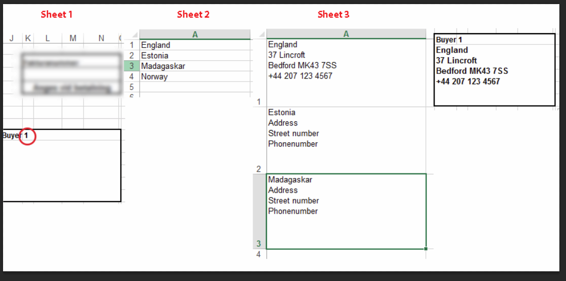
I do have a box in sheet 1 that are merged from many rows and columns, this is where I want the information to end up. By writing a number next to "buyer" I want the program to go to sheet 3, find that number. For example if I look at my list of customers (sheet2) and want england. I write 1 and the program look up 1 in sheet 3 and copy that text to the empty box in sheet 1.
(Sheet number 2 is just a easy list with name in orders so I can find my custumers number easy.
I hope this is possible with index or something. I really want to learn excel more. Hope for answers. BTW using excel 2013

 

[TheGlovner]

Can't see your attachment, but what you are talking about sounds like it would work fine using Index(Match or Vlookup.

 

[vinstic]

Can't you see my picture? http://embed.gyazo.com/af47913c780f22a79e93737404611095.png
Sorry, I'm totaly noob at this. I have heard the name of the methods, but I have no clue how to use them
Tell me if I need to explain more about what I want to do

 

[TheGlovner]

Unfortunately the office network doesn't like the photobucket et al websites.

vlookup is pretty simple. There are four inputs that make up the formula (last one being optional if I remember right), I've split them up below with some plain English explanation:

=vlookup(
             "The Value you are looking for goes here", 
             "The area/range you wish to search goes here (but see note below)", 
             "The number of the column from your area/range you want to return the value from (counted from the left with the left most column being 1), 
             "Whether you want an approximate match (finds the closest value not over the one you are searching for) or exact match, represented by a 0 or 1
            )

With regards to the second input. A lot of people make the mistake of assuming that the search will take place in the entire range passed into the function. In fact it only searches the first, left most column, for the value (first input). Once the value is found it will pass back the value in the corresponding row to the value found for the column number asked for (input 3). The column number is in relation to the range/area you are dealing with. Not the entire worksheet.

 

[vinstic]

I think that can work, but how do I set the vlookup so it searching from a different worksheet?

 

[TheGlovner]

Just click/click and drag.

That's the beauty of excel, once you begin a formula it will let you click on the worksheet to fill in the parts of the formula rather than relying on the user to enter the cell notation correctly by hand.

So type "=vlookup(" into the formula bar and at that point you can click what you want to search for, then type a comma (to tell excel you've moved onto the next part of the formula). Then go and drag a box around the area you want to search and return values from, remember the column your searching has to be the leftmost column of the box you are drawing. Once you have it again add a comma, now you type the number of the column you want to return (can't click this one in as it's a column number in relation to the range you are creating so the excel application doesn't see it as column 1-x the same as you would). Comma again then type FALSE or 0 (it's an boolean so Excel is happy to accept either notation).

It's probably worth putting some dollar signs on the range part of your formula when it's done. It sounds like your pretty new to all this so you need to be aware that when you set cell references without the dollar signs (absolute references) the formula is always in relation to the cell it exists in. So if you copy the formula or move it elsewhere the references will change accordingly so there is the same number of columns and rows between the cell with the formula and the one it references.

Adding the dollar signs means that regardless of where the cell containing the formula is moved to, the cells it actually references remain unchanged.

Other solution to this issue is making good use of named ranges but that's for another day.

 

[vinstic]

Never mind, I solved it with you latest answer!
Thank you so much for the help, I hope I will become better at this ^^