Including more target cells into existing code (VBA)

JBM91

New Member
Joined
Oct 22, 2019
Messages
25
Office Version
  1. 365
Platform
  1. Windows
Hi experts,

So I have this code, which works like a charm for its intended purpose:

VBA Code:
Private Sub Worksheet_Change(ByVal Target As Range)

'Sort planning based on week

Dim cel As Range, Headers As Range
Dim s As String

Set Headers = Range("i1:ABJ1")

If Target.Address = "$G$17" Then
s = Target.Value
Application.ScreenUpdating = False
If s = "" Then
Headers.EntireColumn.Hidden = False

Else

For Each cel In Headers
cel.EntireColumn.Hidden = Not cel.Value = s
Next cel
End If
Application.ScreenUpdating = True

End If

End Sub

However, I would like to have a "sub-version" of this that would then be tied to a button. Other than being a sub and not a worksheet change, it'd also have to either include more target addresses, or, alternatively, also target values that are within -2 of the If Target.Address = "$G$17". E.g. if the

VBA Code:
If Target.Address = "$G$17"
Is set to 5, it'd have to also target headers with 4 and 3 - if that makes sense.

Any tips, tricks or help would be greatly appreciated.
 

Excel Facts

Excel Wisdom
Using a mouse in Excel is the work equivalent of wearing a lanyard when you first get to college
If this code was triggered from a button there would be no Target argument.

What would you want to replace that with?
 
Upvote 0
If this code was triggered from a button there would be no Target argument.

What would you want to replace that with?
I'm open for any ideas and/or recommendations really!
As long as it manages to do what it's supposed to do - any suggestions? :)
 
Upvote 0
What is the code supposed to do?

Is it to hide specific columns based on the value in specific cells?

What other ranges would you want to add to the code?
 
Upvote 0
What is the code supposed to do?

Is it to hide specific columns based on the value in specific cells?

What other ranges would you want to add to the code?
Yeah, but the other way around; it unhides columns in the range I1:ABJ1 that have a header value which corresponds to the value in the target address and hide everything else.
Instead of G17 it would be then be E20, E21 and E22.
 
Upvote 0
Edit.

Confusing phrasing on my part, sorry: It hides all columns in the range I1:ABJ1 that does not have a header value that corresponds to the value in the target address.
 
Upvote 0
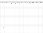
This should do what you want, Starting will cell G17 and working down you can enter column numbers, these references unhide the relevant columns in the workbook:

1579084273039.png


VBA Code:
Sub test()
Dim cel As Range, Headers As Range, columnarr() As Variant, x As Single, rowc As Double
Dim s As String
Set Headers = Range("i1:ABJ1")
Headers.EntireColumn.Hidden = False
lastr = Range("g1000").End(xlUp).Row
rowc = Range(Range("g17"), "g" & lastr).Rows.Count
' Set number of items in array
ReDim columnarr(1 To rowc)
'Array created storing column numbers
columnarr = Application.Transpose(Range(Range("g17"), Range("g" & lastr)))
Application.ScreenUpdating = False
Headers.EntireColumn.Hidden = True
x = 1
'do while unhides columns based on references in column G
Do While x <= UBound(columnarr)
Headers.Cells(1, columnarr(x)).EntireColumn.Hidden = False
x = x + 1
Loop
Application.ScreenUpdating = True
End Sub
 

Attachments

  • 1579084245465.png
    1579084245465.png
    18.8 KB · Views: 2
Upvote 0
This should do what you want, Starting will cell G17 and working down you can enter column numbers, these references unhide the relevant columns in the workbook:

View attachment 4009

VBA Code:
Sub test()
Dim cel As Range, Headers As Range, columnarr() As Variant, x As Single, rowc As Double
Dim s As String
Set Headers = Range("i1:ABJ1")
Headers.EntireColumn.Hidden = False
lastr = Range("g1000").End(xlUp).Row
rowc = Range(Range("g17"), "g" & lastr).Rows.Count
' Set number of items in array
ReDim columnarr(1 To rowc)
'Array created storing column numbers
columnarr = Application.Transpose(Range(Range("g17"), Range("g" & lastr)))
Application.ScreenUpdating = False
Headers.EntireColumn.Hidden = True
x = 1
'do while unhides columns based on references in column G
Do While x <= UBound(columnarr)
Headers.Cells(1, columnarr(x)).EntireColumn.Hidden = False
x = x + 1
Loop
Application.ScreenUpdating = True
End Sub
Hi Tom,

Thanks for the suggestion! I might be wrong, but won't this formula assume that column G is exclusively used for the purpose of cell reference for columns to hide?
In my case, everything below G22 is populated with data. Although I like the idea of having a dynamic formula that'll update when you enter a new value in the G-column, what I need is probably a "static" or fixed reference to cells G20, G21 and G22 only.

Is it possible to alter the formula you provided to do that instead?
 
Upvote 0
This should do what you want, Starting will cell G17 and working down you can enter column numbers, these references unhide the relevant columns in the workbook:

View attachment 4009

VBA Code:
Sub test()
Dim cel As Range, Headers As Range, columnarr() As Variant, x As Single, rowc As Double
Dim s As String
Set Headers = Range("i1:ABJ1")
Headers.EntireColumn.Hidden = False
lastr = Range("g1000").End(xlUp).Row
rowc = Range(Range("g17"), "g" & lastr).Rows.Count
' Set number of items in array
ReDim columnarr(1 To rowc)
'Array created storing column numbers
columnarr = Application.Transpose(Range(Range("g17"), Range("g" & lastr)))
Application.ScreenUpdating = False
Headers.EntireColumn.Hidden = True
x = 1
'do while unhides columns based on references in column G
Do While x <= UBound(columnarr)
Headers.Cells(1, columnarr(x)).EntireColumn.Hidden = False
x = x + 1
Loop
Application.ScreenUpdating = True
End Sub

Hi Tom,

So I tried modifying the formula myself according to the comments I made in my previous reply, please see below:

VBA Code:
Sub test()
Dim cel As Range, Headers As Range, columnarr() As Variant, x As Single, rowc As Double
Dim s As String

Set Headers = Range("I1:ABJ1")

Headers.EntireColumn.Hidden = False
lastr = Range("G22").Row
rowc = Range(Range("G20"), "G" & lastr).Rows.Count

' Set number of items in array
ReDim columnarr(1 To rowc)
'Array created storing column numbers
columnarr = Application.Transpose(Range(Range("G20"), Range("G" & lastr)))
Application.ScreenUpdating = False
Headers.EntireColumn.Hidden = True
    x = 1

    'do while unhides columns based on references in column G
Do While x <= UBound(columnarr)
Headers.Cells(1, columnarr(x)).EntireColumn.Hidden = False
x = x + 1

Loop
Application.ScreenUpdating = True

End Sub

However, when I run it, it seems as if the formula will stop at the K-column and just hide everything past that. When I enter the developer tab and try to run the code in steps, it would appear that the reason is that the macro will only run this part:


VBA Code:
    'do while unhides columns based on references in column G
Do While x <= UBound(columnarr)
Headers.Cells(1, columnarr(x)).EntireColumn.Hidden = False
x = x + 1

Loop
3 times before ending the sub, thereby only "evaluating" the 3 initial columns I, J and K - is there a workaround to that?
 
Last edited:
Upvote 0

Forum statistics

Threads
1,214,976
Messages
6,122,539
Members
449,088
Latest member
RandomExceller01

We've detected that you are using an adblocker.

We have a great community of people providing Excel help here, but the hosting costs are enormous. You can help keep this site running by allowing ads on MrExcel.com.
Allow Ads at MrExcel

Which adblocker are you using?

Disable AdBlock

Follow these easy steps to disable AdBlock

1)Click on the icon in the browser’s toolbar.
2)Click on the icon in the browser’s toolbar.
2)Click on the "Pause on this site" option.
Go back

Disable AdBlock Plus

Follow these easy steps to disable AdBlock Plus

1)Click on the icon in the browser’s toolbar.
2)Click on the toggle to disable it for "mrexcel.com".
Go back

Disable uBlock Origin

Follow these easy steps to disable uBlock Origin

1)Click on the icon in the browser’s toolbar.
2)Click on the "Power" button.
3)Click on the "Refresh" button.
Go back

Disable uBlock

Follow these easy steps to disable uBlock

1)Click on the icon in the browser’s toolbar.
2)Click on the "Power" button.
3)Click on the "Refresh" button.
Go back
Back
Top