Index aggregate or similar formula to return data from another sheet

[the footbal coach]

Looking for a proper formula to find data in another sheet and return adjacent column. Using excel 2016 and 365 at times, but I would like this to work on as many versions as possible.

I need to look up a cell from another sheet and return a value and its adjacent value (if possible, if I need two formulas, I understand). I only have 250 rows or so.

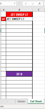
The second picture is Call sheet, I would like to look the data from B1 (jet sweep lt) from the master sheet (picture 1) and return those values back to the call sheet like in the example. Where the formula finds "jet sweep lt" in the master sheet and returns "A1" and "JET SWEEP LT" in the first and second column. (If I had put "JET" in B1, it would have returned A1,A2,A3,A4,A6,A7 etc. down the column.) I have done this with Vlookup, but I could have matching data that needs to return separate row data.

I have seen index match could work, maybe Aggregate to count multiple matches, but I am very out of my element with those functions. I just need to be able to find numbers or words.

This is an example of what my finished sheet looks like currently, but I have recently had trouble with matching data I did not anticipate before.

 

[KRice]

Here is one approach using the INDEX/AGGREGATE approach...

MrExcel20210214.xlsx
	A	B
1		Power
2	A2	Let LT-Power 33
3	A4	Jet LT-Power 33 Pass
4	A5	Power 47-O
5	A12	Power 33
6	A15	Jet RT-Power 34
7	A17	Jet RT-Power 34 Pass
8	A18	Power 28-O
9
10
11
12
13
14
15
16
17
18
19
20
Call Sheet

Cell Formulas
Range	Formula
A2:A20	A2	=IFERROR(INDEX(Master!$A$2:$B$21,AGGREGATE(15,6,(ROW(Master!$B$2:$B$21)-ROW('Call Sheet'!$B$1))/ISNUMBER(SEARCH('Call Sheet'!$B$1,Master!$B$2:$B$21)),ROWS(A$2:A2)),1),"")
B2:B20	B2	=IFERROR(INDEX(Master!$A$2:$B$21,AGGREGATE(15,6,(ROW(Master!$B$2:$B$21)-ROW('Call Sheet'!$B$1))/ISNUMBER(SEARCH('Call Sheet'!$B$1,Master!$B$2:$B$21)),ROWS(B$2:B2)),2),"")

MrExcel20210214.xlsx
	A	B
1
2	A1	Jet Sweep LT
3	A2	Let LT-Power 33
4	A3	Jet LT-24 OT
5	A4	Jet LT-Power 33 Pass
6	A5	Power 47-O
7	A6	Jet LT-31 Trap
8	A7	Jet LT-35 G
9	A8	Jet LT-24 Counter
10	A9	Jet LT-35 G Pass
11	A10	35 Down
12	A11	Jet LT-35 G Pass Switch
13	A12	Power 33
14	A13	Jet LT-35 G Pass Y-Cross
15	A14	Jet Sweep RT
16	A15	Jet RT-Power 34
17	A16	Jet RT-43 OT
18	A17	Jet RT-Power 34 Pass
19	A18	Power 28-O
20	A19	Jet RT-32 Trap
21	A20	Jet RT-36 G
Master

 

[the footbal coach]

Thank You very much. I think Its working perfectly. My conditional formatting is messing up, but this has been a life saver. Thank you again

 

[KRice]

Glad to help. Post back if you run into issues with the conditional formatting. It looks as if you might want to fill cells depending on the first letter of the play's index code...with "A" filled red with white font, "C" filled blue with white font, etc. If that is true, then conditional formatting based on a formula should work, =LEFT(cell reference,1)...as shown in this example.

MrExcel20210214.xlsx
	A	B
1		LT
2	A1	Jet Sweep LT
3	A2	Let LT-Power 33
4	A3	Jet LT-24 OT
5	A4	Jet LT-Power 33 Pass
6	A6	Jet LT-31 Trap
7	A7	Jet LT-35 G
8	A8	Jet LT-24 Counter
9	A9	Jet LT-35 G Pass
10	A11	Jet LT-35 G Pass Switch
11	A13	Jet LT-35 G Pass Y-Cross
12	C13	Jet Sweep LT
13	C14	Jet LT-Power 33
14
15
16
17
18
19
20
Call Sheet

Cell Formulas
Range	Formula
A2:A20	A2	=IFERROR(INDEX(Master!$A$2:$B$25,AGGREGATE(15,6,(ROW(Master!$B$2:$B$25)-ROW('Call Sheet'!$B$1))/ISNUMBER(SEARCH('Call Sheet'!$B$1,Master!$B$2:$B$25)),ROWS(A$2:A2)),1),"")
B2:B20	B2	=IFERROR(INDEX(Master!$A$2:$B$25,AGGREGATE(15,6,(ROW(Master!$B$2:$B$25)-ROW('Call Sheet'!$B$1))/ISNUMBER(SEARCH('Call Sheet'!$B$1,Master!$B$2:$B$25)),ROWS(B$2:B2)),2),"")

Cells with Conditional Formatting
Cell	Condition		Cell Format	Stop If True
A2:A20	Expression	=LEFT(A2,1)="C"	text	NO
A2:A20	Expression	=LEFT(A2,1)="A"	text	NO

 

[the footbal coach]

I think everything has worked out great. The formula was making all my conditional formatting selections delete, just fixed those and everything is great. thank you again

 

[KRice]

Good to hear...thanks for the update.