Index and Match with multiple criteria

[Indominus]

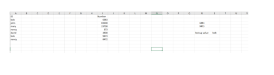
Hello. The attached photo is just an example. So I have this workbook that has multiple sheets like this where I would have to run the same type of code. In one sheet I have at least two lookup values. Another sheet I have a file like the one attached. Referenced as Raw data. One lookup value which will be a person’s username will be in column A. I then have at least two numbers that I need to identify if the username has them attached. These are in column I in Raw data sheet. In the real sheet the lookup values, the username and two numbers, won’t be in column R but in my main sheet. If that matters. But what I need to be able to do is for example, is find
IF Bob has both 6383 and 9473, “pass”,”fail”. Basically an IF formula with this.

I have tried Index and match but it won’t work straight up since it will only find the first time Bob appears. I YouTubed this and it seems maybe I will have to use arrays or the small formula. Not 100% sure though. Any help would be very appreciated. Thank you in advance!

 

[Marcelo Branco]

Try

=IF((COUNTIFS(A:A,"bob",I:I,6383)>0)+(COUNTIFS(A:A,"bob",I:I,9473)>0)=2,"pass","fail")

M.

 

[Marcelo Branco]

Using cell references
=IF((COUNTIFS(A:A,S6,I:I,R3)>0)+(COUNTIFS(A:A,S6,I:I,R4)>0)=2,"pass","fail")

M.

 

[DanteAmor]

Another way:

=IF(SUMPRODUCT((A2:A20=S6)*((I2:I20=R3)+(I2:I20=R4)))=2,"pass","fail")

Note: You must limit the range of cells

 

[Marcelo Branco]

Dante,
I think your formula doesn't give the correct result if there are two instances Bob - 6383 (or Bob - 9473)

M.

 

[DanteAmor]

I think your formula doesn't give the correct result if there are two instances Bob - 6383 (or Bob - 9473)

Ah ok.Then

Dante Amor.xlsm
	A	B							I	J								R	S	T
1	Id
2	bob								6383											Pass
3	john								83638									6383		Pass
4	mary								23738									9473
5	nancy								373
6	bob								9473										bob
7	bob								9473
8	nancy								8472
Hoja6

Cell Formulas
Range	Formula
T2	T2	=IF(SUMPRODUCT((A2:A20=S6)*((I2:I20=R3)+(I2:I20=R4)))>=2,"Pass","Fail")
T3	T3	=IF(COUNTIFS(A:A,S6,I:I,R3)+COUNTIFS(A:A,S6,I:I,R4)>=2,"Pass","Fail")

 

[Marcelo Branco]

Pasta1
	A	B	C	D	E	F	G	H	I
1	ID		My Formula	Your Formula					Number
2	bob		fail	pass					6383
3	john								83638
4	may								23738
5	nancy								373
6	david								3838
7	bob								6383
8	nancy								8472
Plan3

Cell Formulas
Range	Formula
C2	C2	=IF((COUNTIFS(A:A,"bob",I:I,6383)>0)+(COUNTIFS(A:A,"bob",I:I,9473)>0)=2,"pass","fail")
D2	D2	=IF(SUMPRODUCT((A2:A20=S6)*((I2:I20=R3)+(I2:I20=R4)))=2,"pass","fail")

M.

 

[DanteAmor]

Thanks, I already saw it. Then

=IF(SUMPRODUCT((A2:A20=S6)*((I2:I20=R3)+(I2:I20=R4)))>=2,"Pass","Fail")

Or

=IF(COUNTIFS(A:A,S6,I:I,R3)+COUNTIFS(A:A,S6,I:I,R4)>=2,"Pass","Fail")

 

[Marcelo Branco]

I don't know if such a scenario is possible in the real case, but we are still getting different results

Pasta1
	A	B	C	D	E	F	G	H	I
1	ID		My Formula	Your New F1	Your New F2				Number
2	bob		fail	Pass	Pass				6383
3	john								83638
4	may								23738
5	nancy								373
6	david								3838
7	bob								6383
8	nancy								8472
Plan3

Cell Formulas
Range	Formula
C2	C2	=IF((COUNTIFS(A:A,S6,I:I,R3)>0)+(COUNTIFS(A:A,S6,I:I,R4)>0)=2,"pass","fail")
D2	D2	=IF(SUMPRODUCT((A2:A20=S6)*((I2:I20=R3)+(I2:I20=R4)))>=2,"Pass","Fail")
E2	E2	=IF(COUNTIFS(A:A,S6,I:I,R3)+COUNTIFS(A:A,S6,I:I,R4)>=2,"Pass","Fail")

M.

 

[DanteAmor]

You are right, it is a case and if it is presented my formula is not correct.
Also your formula is faster, I vote for your formula. Thanks for comment.