Index Match Date N/A

[jcmac]

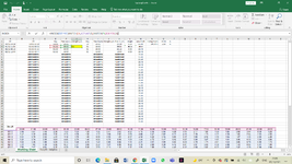
I am trying to use index match but cannot get it to work, it works when I manually enter the time and date into the cells next to the yellow box but when using the formula ref i get n/a error.

Indext Match Formula

=INDEX(B37:Y67,MATCH(E4,A37:A67,0),MATCH(F4,B36:Y36,0))

 

[Phuoc]

Try this:

=INDEX(B37:Y67,MATCH(E4,A37:A67,0),HOUR(F4)+1)

 

[Alex Blakenburg]

If Phuoc's suggestion doesn't work, then themost likely issue is that the formulas used are not returning a date value or time value but text. Or the date part is not including the year and defaulting to a different year.
Start with supplying us with an XL2BB so we can actually see what you have in the cells.

 

[jcmac]

SailingDrafts (2).xlsx
	A	B	C	D	E	F	G	H	I	J	K	L	M	N	O
1			HW -2 Hours			Tide
2	DT		DT		Date x1	Time A (x1)	A height (y1)	Time B (x3)	B height (y3)	Time C (x2)	Height	Max Draft	Ruling Depth	18.50	m
3	30/11 23:20		30/11 21:20		30/11	21:00		22:00		21:20	0.00	16.40	UKC Min	2.10	m
4	01/12 11:44		01/12 09:44		01/12	9:00		10:00		9:44	0.00	16.40
5	02/12 00:12		01/12 22:12		01/12	22:00		23:00		22:12	0.00	16.40
6	02/12 12:43		02/12 10:43		02/12	10:00		11:00		10:43	0.00	16.40
7	03/12 01:02		02/12 23:02		02/12	23:00		0:00		23:02	0.00	16.40
8	03/12 13:29		03/12 11:29		03/12	11:00		12:00		11:29	0.00	16.40
Working Sheet

Cell Formulas
Range	Formula
E3:E8	E3	=F3
F3:F8	F3	=FLOOR(C3,TIME(1,0,0))
J3:J8	J3	=C3
K3:K8	K3	=SUM(((J3-F3)*(I3-G3))/(H3-F3))+G3
L3:L8	L3	=SUM(18.5+K3-2.1)
C3:C8	C3	=SUM(A3-(2/24))
H3:H8	H3	=CEILING(C3,TIME(1,0,0))

SailingDrafts (2).xlsx
	A	B	C	D	E	F	G	H	I	J	K	L	M	N	O	P	Q	R	S	T	U	V	W	X	Y
1	Dec-21
2	0	0:00	1:00	2:00	3:00	4:00	5:00	6:00	7:00	8:00	9:00	10:00	11:00	12:00	13:00	14:00	15:00	16:00	17:00	18:00	19:00	20:00	21:00	22:00	23:00
3	1	5.04	4.47	3.46	2.36	1.63	1.33	1.28	1.65	2.47	3.53	4.52	5.15	5.34	5.04	4.24	3.14	2.17	1.69	1.59	1.85	2.60	3.64	4.59	5.20
4	2	5.47	5.32	4.59	3.35	2.05	1.28	1.05	1.07	1.56	2.63	3.89	4.88	5.47	5.62	5.17	4.13	2.78	1.71	1.32	1.30	1.65	2.64	3.93	4.93
5	3	5.51	5.76	5.52	4.59	3.12	1.70	1.00	0.86	0.95	1.63	2.97	4.32	5.22	5.74	5.80	5.17	3.86	2.32	1.30	1.04	1.07	1.55	2.80	4.26
6	4	5.21	5.74	5.98	5.61	4.46	2.79	1.40	0.86	0.79	0.96	1.89	3.44	4.72	5.47	5.92	5.87	5.00	3.47	1.87	1.01	0.86	0.93	1.58	3.06
7	5	4.52	5.36	5.88	6.09	5.56	4.20	2.48	1.23	0.85	0.82	1.13	2.31	3.91	4.99	5.60	6.00	5.79	4.71	3.04	1.53	0.86	0.78	0.90	1.73
8	6	3.31	4.64	5.38	5.92	6.07	5.37	3.89	2.23	1.21	0.96	0.98	1.46	2.80	4.28	5.12	5.64	5.97	5.59	4.36	2.68	1.33	0.85	0.81	1.00
9	7	1.95	3.47	4.61	5.30	5.86	5.91	5.09	3.60	2.11	1.32	1.17	1.25	1.89	3.24	4.49	5.12	5.58	5.82	5.32	4.02	2.42	1.29	0.96	0.94
Heights

Cell Formulas
Range	Formula
A4:A9	A4	=SUM(A3+1)

 

[mackc557]

With your original posted picture there shouldn't be any reason it's not working. However with your sample, the numbers under the Dec-21 are just integers, not dates.

 

[jcmac]

I have been looking more and narrowed the issue down to the date field in column E. If the date is extracted from the column H it doesn't work, but if entered manually good.

SailingDrafts (2).xlsx
	A	B	C	D	E	F	G	H	I	J	K	L	M	N	O
1			HW -2 Hours			Tide
2	DT		DT		Date x1	Time A (x1)	A height (y1)	Time B (x3)	B height (y3)	Time C (x2)	Height	Max Draft	Ruling Depth	18.50	m
3	30/11 23:20		30/11 21:20		30/11	21:00		22:00		21:20	0.00	16.40	UKC Min	2.10	m
4	01/12 11:44		01/12 09:44		01/12	9:00	3.53	10:00		9:44	0.94	17.34
5	02/12 00:12		01/12 22:12		01/12	22:00	#N/A	23:00		22:12	#N/A	#N/A
6	02/12 12:43		02/12 10:43		02/12	10:00		11:00		10:43	0.00	16.40
Working Sheet

Cell Formulas
Range	Formula
E3,E5:E6	E3	=F3
F3:F6	F3	=FLOOR(C3,TIME(1,0,0))
J3:J6	J3	=C3
K3:K6	K3	=SUM(((J3-F3)*(I3-G3))/(H3-F3))+G3
L3:L6	L3	=SUM(18.5+K3-2.1)
G4:G5	G4	=INDEX(' Heights'!$B$3:$Y$33,MATCH(E4,' Heights'!$A$3:$A$33,0),HOUR(F4)+1)
C3:C6	C3	=SUM(A3-(2/24))
H3:H6	H3	=CEILING(C3,TIME(1,0,0))

SailingDrafts (2).xlsx
	A	B	C	D	E	F	G	H	I	J	K	L	M	N	O
1			HW -2 Hours			Tide
2	DT		DT		Date x1	Time A (x1)	A height (y1)	Time B (x3)	B height (y3)	Time C (x2)	Height	Max Draft	Ruling Depth	18.50	m
3	30/11 23:20		30/11 21:20		30/11	21:00		22:00		21:20	0.00	16.40	UKC Min	2.10	m
4	01/12 11:44		01/12 09:44		01/12	9:00	3.53	10:00		9:44	0.94	17.34
5	02/12 00:12		01/12 22:12		01/12	22:00	4.59	23:00		22:12	3.67	20.07
6	02/12 12:43		02/12 10:43		02/12	10:00		11:00		10:43	0.00	16.40
Working Sheet

Cell Formulas
Range	Formula
E3,E6	E3	=F3
F3:F6	F3	=FLOOR(C3,TIME(1,0,0))
J3:J6	J3	=C3
K3:K6	K3	=SUM(((J3-F3)*(I3-G3))/(H3-F3))+G3
L3:L6	L3	=SUM(18.5+K3-2.1)
G4:G5	G4	=INDEX(' Heights'!$B$3:$Y$33,MATCH(E4,' Heights'!$A$3:$A$33,0),HOUR(F4)+1)
C3:C6	C3	=SUM(A3-(2/24))
H3:H6	H3	=CEILING(C3,TIME(1,0,0))

 

[Alex Blakenburg]

With your original posted picture there shouldn't be any reason it's not working. However with your sample, the numbers under the Dec-21 are just integers, not dates.

Following on from mack's comment, try this in G3

=INDEX(Heights!$B$3:$Y$33,MATCH(DAY(E3),Heights!$A$3:$A$33,0),HOUR(F3)+1)

 

[AhoyNC]

If you just want a date (no time) in column E then try changing your formula to:
=INT(F3)

If you remove the formatting from your sheet you will notice that the time portion of your formulas are not finding a match due to the time (decimal part) of your formula not matching because of the FLOOR function. See below

Book1
	A	B	C	D	E	F	G	H
1			HW -2 Hours			Tide
2	DT		DT		Date x1	Time A (x1)	A height (y1)	Time B (x3)
3	44530.97222		44530.88889		44530.875	44530.875		44530.91667
4	44531.48889		44531.40556		44531	44531.375	#N/A	44531.41667
5	44532.00833		44531.925		44531.91667	44531.91667	#N/A	44531.95833
6	44532.52986		44532.44653		44532.41667	44532.41667		44532.45833
Sheet1

Cell Formulas
Range	Formula
E3,E5:E6	E3	=F3
F3:F6	F3	=FLOOR(C3,TIME(1,0,0))
G4:G5	G4	=INDEX(' Heights'!$B$3:$Y$33,MATCH(E4,' Heights'!$A$3:$A$33,0),HOUR(F4)+1)
C3:C6	C3	=SUM(A3-(2/24))
H3:H6	H3	=CEILING(C3,TIME(1,0,0))

 

[jcmac]

If you just want a date (no time) in column E then try changing your formula to:
=INT(F3)

Solved - thanks for your help really appreciate it.

 

[AhoyNC]

You're welcome. Thanks for the feedback.