Index Match Date Range for Invoices

[IanPayroll]

Hi,

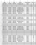
I'm trying to create Invoices for multiple clients from a master list of daily work performed.
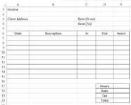
I would like to be able to enter a single client address on an Invoice Sheet (currently 'Sheet2!$b$3') & Date From: (Sheet2!$d$3) & Date To (Sheet2!$d$4).
I would like excel to auto populate all the information for that client for work completed in that date range. ("Date", "Description", "In", "Out", "Hours")

Sheet1! is the Master List & Sheet2! is the Invoice Sheet

I was thinking it would be a Index Match If And Formula Looking something like:

=INDEX(Sheet1!$a$2:$a$32(MATCH(Sheet2!$b$3,Sheet1!$d$2:$d$32,0)) (to get the date from Sheet 1) - Then INDEX(Sheet1!$e$2:$e$32...) (to get Description); Then INDEX(Sheet1!$b$2:$b$32...) (to get "In"); and "Then INDEX(Sheet1!$c$2:$c$32...) (to get "Out")

I would use the relevant formulas to fill hours, rate, tax and total

I've tried adding a variety of IF AND formulas but I'm stumped at how to only pull data from a date range for a single client. Can anyone offer some suggestions? I'm sure it's really easy but I'm just not able to figure it out.

Thanks in advance.

 

[Toadstool]

Hi Ianpayroll,

Try this. Here's your data in Sheet1

IanPayroll.xlsx
	A	B	C	D	E	F
1	Date	In	Out	Client	Description	Hours
2	2021 01 01	7:00 AM	5:00 PM	123 Acacia Ave	Task1	10
3	2021 01 02	7:00 AM	4:30 PM	2 Browns Rd	Task2	9.5
4	2021 01 03	7:30 AM	5:00 PM	44 Clutch St	Task3	9.5
5	2021 01 04					0
6	2021 01 05					0
7	2021 01 06	7:00 AM	5:00 PM	123 Acacia Ave	Task6	10
8	2021 01 07	7:00 AM	5:00 PM	2 Browns Rd	Task7	10
9	2021 01 08	7:30 AM	4:30 PM	2 Browns Rd	Task8	9
10	2021 01 09	7:30 AM	6:15 PM	2 Browns Rd	Task9	10.75
11	2021 01 10	7:00 AM	5:00 PM	44 Clutch St	Task10	10
12	2021 01 11					0
13	2021 01 12					0
14	2021 01 13	7:00 AM	5:00 PM	123 Acacia Ave	Task13	10
15	2021 01 14	7:30 AM	4:30 PM	2 Browns Rd	Task14	9
16	2021 01 15	7:00 AM	5:00 PM	2 Browns Rd	Task15	10
Sheet1

Cell Formulas
Range	Formula
F2:F16	F2	=(C2-B2)*24

Here's your invoice page:

IanPayroll.xlsx
	A	B	C	D	E
1	Invoice
2
3	Client Address	2 Browns Rd	Date From:	2021 01 03
4			Date To:	2021 01 14
5
6	Date	Description	In	Out	Hours
7	2021 01 07	Task7	7:00 AM	5:00 PM	10
8	2021 01 08	Task8	7:30 AM	4:30 PM	9
9	2021 01 09	Task9	7:30 AM	6:15 PM	10.75
10	2021 01 14	Task14	7:30 AM	4:30 PM	9
11
12
13
14
15
16
17				Hours	38.75
18				Rate
19				Tax
20				Total
Sheet2

Cell Formulas
Range	Formula
A7:A15	A7	=IFERROR(INDEX(Sheet1!$A$2:$A$9999,AGGREGATE(15,6,ROW(Sheet1!$A$2:$A$9999)-ROW(Sheet1!$A$1)/((Sheet1!$D$2:$D$9999=$B$3)*(Sheet1!$A$2:$A$9999>=$D$3)*(Sheet1!$A$2:$A$9999<=$D$4)),ROW()-ROW($A$6))),"")
B7:B15	B7	=IFERROR(INDEX(Sheet1!$E$2:$E$9999,AGGREGATE(15,6,ROW(Sheet1!$A$2:$A$9999)-ROW(Sheet1!$A$1)/((Sheet1!$D$2:$D$9999=$B$3)*(Sheet1!$A$2:$A$9999>=$D$3)*(Sheet1!$A$2:$A$9999<=$D$4)),ROW()-ROW($A$6))),"")
C7:D15	C7	=IFERROR(INDEX(Sheet1!B$2:B$9999,AGGREGATE(15,6,ROW(Sheet1!$A$2:$A$9999)-ROW(Sheet1!$A$1)/((Sheet1!$D$2:$D$9999=$B$3)*(Sheet1!$A$2:$A$9999>=$D$3)*(Sheet1!$A$2:$A$9999<=$D$4)),ROW()-ROW($A$6))),"")
E7:E15	E7	=IFERROR(INDEX(Sheet1!$F$2:$F$9999,AGGREGATE(15,6,ROW(Sheet1!$A$2:$A$9999)-ROW(Sheet1!$A$1)/((Sheet1!$D$2:$D$9999=$B$3)*(Sheet1!$A$2:$A$9999>=$D$3)*(Sheet1!$A$2:$A$9999<=$D$4)),ROW()-ROW($A$6))),"")
E17	E17	=SUM(E7:E15)

 

[IanPayroll]

That's exactly what I was looking for. Thank you very much for taking the time to write all that out. I really appreciate it Toadstool.

 

[Toadstool]

That's exactly what I was looking for. Thank you very much for taking the time to write all that out. I really appreciate it Toadstool.

You're welcome!
Thanks for the feedback.

 

[Peter_SSs]

Just a suggestion. Using the same concept Toadstool has used, you could simplify the majority of the formulas and reduce the amount of calculations required considerably by using a helper column.
Here I have used column F in Sheet2 (Sheet1 is identical to Toadstool's Sheet1) as the helper column and that column could be hidden once you enter the formulas.

IanPayroll.xlsm
	A	B	C	D	E	F
1	Invoice
2
3	Client Address	2 Browns Rd	Date From:	2021 01 03
4			Date To:	2021 01 14
5
6	Date	Description	In	Out	Hours
7	2021 01 07	Task7	7:00 AM	5:00 PM	10	7
8	2021 01 08	Task8	7:30 AM	4:30 PM	9	8
9	2021 01 09	Task9	7:30 AM	6:15 PM	10.75	9
10	2021 01 14	Task14	7:30 AM	4:30 PM	9	14
11						0
12						0
13						0
14						0
15						0
16
17				Hours	38.75
18				Rate
19				Tax
20				Total
Sheet2

Cell Formulas
Range	Formula
A7:A15	A7	=IF(F7,INDEX(Sheet1!$A$2:$A$9999,F7),"")
B7:B15	B7	=IF(F7,INDEX(Sheet1!$E$2:$E$9999,F7),"")
C7:C15	C7	=IF(F7,INDEX(Sheet1!B$2:B$9999,F7),"")
D7:D15	D7	=IF(F7,INDEX(Sheet1!C$2:C$9999,F7),"")
E7:E15	E7	=IF(F7,INDEX(Sheet1!$F$2:$F$9999,F7),"")
F7:F15	F7	=IFERROR(AGGREGATE(15,6,ROW(Sheet1!$A$2:$A$9999)-ROW(Sheet1!$A$1)/((Sheet1!$D$2:$D$9999=$B$3)*(Sheet1!$A$2:$A$9999>=$D$3)*(Sheet1!$A$2:$A$9999<=$D$4)),ROW()-ROW($F$6)),0)
E17	E17	=SUM(E7:E15)