Index Match formula or one better that solves this problem ....(No VBA)

[gotido]

Hello,

I´m trying to create a file where I can put data that I export from a company software, which gives me the sales items for each commercial and the value.

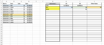
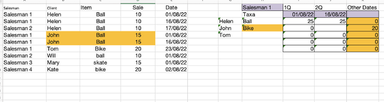
In a table I would like to get the values of each item, that correspond to a specific commercial and that the item is placed in the sales dates.
The sales that coincided with Q1 would be in Q1 and the same for Q2.
All sales outside of these dates would be in the other sales.

Is this possible using just formulas?

 

[Peter_SSs]

Any chance that you could give us the sample data with XL2BB so that we can easily copy to test with?

 

[jorismoerings]

Hi,

Something like this:

Book1
	A	B	C	D	E	F	G	H	I	J
1	Name	Item	Sale	Date			Salesman 1	1Q	2Q	Other Dates
2	Salesman 1	ball	10	1-8-2022			Item	1-8-2022	16-8-2022
3	Salesman 1	skate	12	16-8-2022			ball	10	16	14
4	Salesman 2	bike	15	1-8-2022			skate	0	12	0
5	Salesman 3	skate	11	1-8-2022
6	Salesman 4	skate	10	2-8-2022
7	Salesman 1	ball	14	10-8-2022
8	Salesman 1	ball	16	16-8-2022
9	Salesman 2	bike	12	1-8-2022
10	Salesman 3	skate	14	16-8-2022
11	Salesman 4	skate	16	16-8-2022
Sheet2

Cell Formulas
Range	Formula
G3:G4	G3	=UNIQUE(FILTER(B2:B11,A2:A11=G1))
H3:I4	H3	=IFERROR(SUM(FILTER($C$2:$C$11,$A$2:$A$11&$D$2:$D$11&$B$2:$B$11=$G$1&H$2&$G3)),0)
J3:J4	J3	=IFERROR(SUM(FILTER($C$2:$C$11,$A$2:$A$11&$B$2:$B$11=$G$1&$G3)),0)-SUM(H3:I3)
Dynamic array formulas.

 

[Peter_SSs]

@jorismoerings

• Thanks for creating the data.
• There is no need for IFERROR in your formula as FILTER allows for a value if nothing is returned from the FILTER. For example, instead of H3 being
  =IFERROR(SUM(FILTER($C$2:$C$11,$A$2:$A$11&$D$2:$D$11&$B$2:$B$11=$G$1&H$2&$G3)),0) it could be
  =SUM(FILTER($C$2:$C$11,$A$2:$A$11&$D$2:$D$11&$B$2:$B$11=$G$1&H$2&$G3,0))

Another set of options

22 08 23.xlsm
	A	B	C	D	E	F	G	H	I	J
1	Name	Item	Sale	Date			Salesman 1	1Q	2Q	Other Dates
2	Salesman 1	ball	10	1/08/2022			Item	1/08/2022	16/08/2022
3	Salesman 1	skate	12	16/08/2022			ball	10	16	14
4	Salesman 2	bike	15	1/08/2022			skate	0	12	0
5	Salesman 3	skate	11	1/08/2022
6	Salesman 4	skate	10	2/08/2022
7	Salesman 1	ball	14	10/08/2022
8	Salesman 1	ball	16	16/08/2022
9	Salesman 2	bike	12	1/08/2022
10	Salesman 3	skate	14	16/08/2022
11	Salesman 4	skate	16	16/08/2022
Q

Cell Formulas
Range	Formula
G3:G4	G3	=UNIQUE(FILTER(B2:B11,A2:A11=G1))
H3:I4	H3	=SUMIFS($C$2:$C$11,$A$2:$A$11,$G$1,$B$2:$B$11,$G3,$D$2:$D$11,H$2)
J3:J4	J3	=SUMIFS(C$2:C$11,A$2:A$11,G$1,B$2:B$11,G3)-SUM(H3:I3)
Dynamic array formulas.

 

[gotido]

Thank you so much!
It worked like a charm!!!

 

[gotido]

I was missing one column, the client..

I tried to fix the formula but i wasn't able to do it...

when two different clients have the same item, the value goes to the wrong place. I put in orange, the places where the formula doesnt work...

Could you please help me?

 

[jorismoerings]

Hi,

try this as a result of my work as well as @Peter_SSs

EF - dependent drop down.xlsx
	A	B	C	D	E	F	G	H	I	J	K	L	M	N	O	P	Q
1	Name	client	Item	Sale	Date		Salesman 1		1Q	2Q	Other Dates		Salesman 1		1Q	2Q	Other Dates
2	Salesman 1	Helen	ball	10	1-8-2022		Client	Item	1-8-2022	16-8-2022			Client	Item	1-8-2022	16-8-2022
3	Salesman 1	Helen	ball	10	16-8-2022		Helen	ball	10	10	0		Helen	ball	10	10	0
4	Salesman 2	Helen	ball	10	17-8-2022		John	ball	15	15	0		John	ball	15	15	0
5	Salesman 1	John	ball	15	1-8-2022		Tom	bike	0	0	20		Tom	bike	0	0	20
6	Salesman 1	John	ball	15	16-8-2022		Will	ball	10	0	0		Will	ball	10	0	0
7	Salesman 1	Tom	bike	20	23-8-2022
8	Salesman 1	Will	ball	10	1-8-2022
9	Salesman 2	Mary	skate	15	1-8-2022
10	Salesman 3	Kate	bike	20	2-8-2022
Sheet1

Cell Formulas
Range	Formula
G3:H6,M3:N6	G3	=UNIQUE(FILTER($B$2:$C$10,$A$2:$A$10=G$1))
I3:J6	I3	=SUMIFS($D$2:$D$10,$A$2:$A$10,$G$1,$C$2:$C$10,$H3,$E$2:$E$10,I$2,$B$2:$B$10,$G3)
K3:K6	K3	=SUMIFS(D$2:D$10,A$2:A$10,G$1,C$2:C$10,H3,$B$2:$B$10,$G3)-SUM(I3:J3)
O3:P6	O3	=SUM(FILTER($D$2:$D$10,$A$2:$A$10&$B$2:$B$10&$C$2:$C$10&$E$2:$E$10=$M$1&$M3&$N3&O$2,0))
Q3:Q6	Q3	=SUM(FILTER($D$2:$D$10,$A$2:$A$10&$B$2:$B$10&$C$2:$C$10=$M$1&$M3&$N3,0))-SUM(O3:P3)
Dynamic array formulas.

As a tip: try to breakdown our proposed solution and try to understand how we came to this solution and if not, ask us to explain. This way you'll gain knowledge on we've used Excel.

 

[gotido]

Ok, i will look at the formula to try to understand it and if i have any doubts i´ll come back to ask for info..Thanks!

 

[gotido]

In the cell K3 it returns the value 0 because ti gives you the sum of 20 and subtracts the same value. is there a way the it recognizes the date diferent than Q1 and Q2 and return the exact value?

 

[gotido]

Found the mistake... the name of the salesman was wrong