Hi, I am hoping someone can help me understand what I am doing wrong and help point me in the right direction...
I have a very large spreadsheet with a number of sheets. One of these sheets is to draw information from another one and I am having some difficulty getting the information I am wanting. After researching the formulas that are possible I believe the index/match formula would be the one to use, however, I am either not understanding it properly or entering it all wrong.
This is what I am trying to acheive:
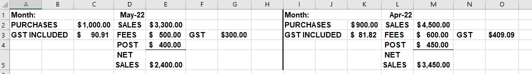
Sheet A: Monthly sales/purchase data (always changing as new months are added to the sheet)
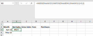
Sheet B: Yearly figures
Sheet A works horizontally with new months pushing the old to the right as they are added and includes totals for each month of "net sales", "gross sales", "GST", "purchases" etc.
So... for example, how can I return the value of "Sales" (4500) for the month of April 22 to SHEET B? I am wanting Sheet B to automatically populate with the information rather than me having to manually enter every figure in each month. I have attached an example of what I am trying to do and tried using the index/match formula as follows:
=INDEX(SheetA!2:5,MATCH(SheetB!A3,SheetA!1:1)+3,2)
(I did try to upload a minisheet- but was unable to so I do hope the images are okay).
Thanks in advance for anyone who can help with this.
I have a very large spreadsheet with a number of sheets. One of these sheets is to draw information from another one and I am having some difficulty getting the information I am wanting. After researching the formulas that are possible I believe the index/match formula would be the one to use, however, I am either not understanding it properly or entering it all wrong.
This is what I am trying to acheive:
Sheet A: Monthly sales/purchase data (always changing as new months are added to the sheet)
Sheet B: Yearly figures
Sheet A works horizontally with new months pushing the old to the right as they are added and includes totals for each month of "net sales", "gross sales", "GST", "purchases" etc.
So... for example, how can I return the value of "Sales" (4500) for the month of April 22 to SHEET B? I am wanting Sheet B to automatically populate with the information rather than me having to manually enter every figure in each month. I have attached an example of what I am trying to do and tried using the index/match formula as follows:
=INDEX(SheetA!2:5,MATCH(SheetB!A3,SheetA!1:1)+3,2)
(I did try to upload a minisheet- but was unable to so I do hope the images are okay).
Thanks in advance for anyone who can help with this.
")


