Index-Match Function - Second match needed

[tt333]

Hi Folks

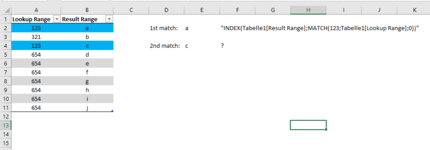
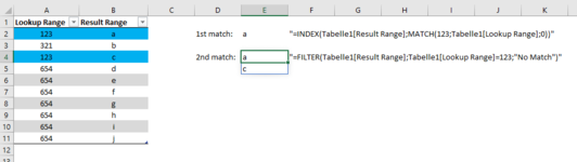
I'm using the INDEX function in combination with the MATCH function on a table (see attached sample), which is straight forward easy. But now i want to find a second match in case there is one.

My attempt was to use OFFSET for the INDEX range (using the MATCH result + 1), but I just fail to get a range in return. OFFSET gives me a SPILL error.

So, in my sample table, I need to adjust the range for the 2nd INDEX MATCH to "A3:A11" instead of Tabelle1[Result Range] (i.e. "A2:A11")

Any ideas?

 

[Fluff]

What version of Excel are you using?

I suggest that you update your Account details (or click your user name at the top right of the forum) so helpers always know what Excel version(s) & platform(s) you are using as the best solution often varies by version. (Don’t forget to scroll down & ‘Save’)

As you are getting a #SPILL error you should have the Filter function, that will return all matches.

 

[jasonb75]

If you're getting a SPILL error then you must have dynamic array functions so should be able to use FILTER

=FILTER(Tabelle1[Result Range];Tabelle1[Lookup Range]=123;"No Match")

 

[tt333]

What version of Excel are you using?

I suggest that you update your Account details (or click your user name at the top right of the forum) so helpers always know what Excel version(s) & platform(s) you are using as the best solution often varies by version. (Don’t forget to scroll down & ‘Save’)

As you are getting a #SPILL error you should have the Filter function, that will return all matches.

Im using the latest 356 version ... I've just updated my account info

 

[Fluff]

Thanks for that, give Jason's formula a try.

 

[tt333]

If you're getting a SPILL error then you must have dynamic array functions so should be able to use FILTER

=FILTER(Tabelle1[Result Range];Tabelle1[Lookup Range]=123;"No Match")

Thank you, that's already a start. The result is an array...but how do I get only the second match

 

[Fluff]

How about

=INDEX(FILTER(Tabelle1[Result Range];Tabelle1[Lookup Range]=123;"No Match");2)

 

[jasonb75]

The result is an array...but how do I get only the second match

You don't need a formula for the second match, use the formula that I suggested for the first match. When there are 2 (or more) matches it will list all of them automatically.

 

[tt333]

How about

=INDEX(FILTER(Tabelle1[Result Range];Tabelle1[Lookup Range]=123;"No Match");2)

Thanks a lot...that does the trick

 

[Fluff]

Glad we could help & thanks for the feedback.