Index & Match in VBA

bhalbach

Board Regular
Joined
Mar 15, 2018
Messages
221
Office Version
  1. 2016
Platform
  1. Windows
How do I convert the following formula to index match in VBA? I cannot wrap my head around this...I am trying to learn but im struggling.

=INDEX(rngLabourRates,MATCH(D13,rngLabour),0)

I have made the following vlookup code work to accomplish what i want but it returns an error when there is a blank in D13:D27 range of TskSheet.
Sub VlookupLabourRate()

For i = 13 To 27
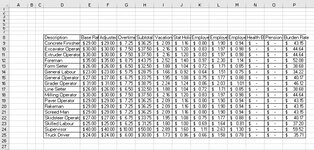
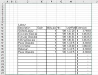
Worksheets("TskSheet").Cells(i, 8).Value = Application.WorksheetFunction.VLookup(Worksheets("TskSheet").Cells(i, 4).Value, Worksheets("Labour").Range("D:P"), 13, 0)
Next

End Sub

I think that Index Match is what I should be using but I am open to any suggestions on how to do this so it returns my results very quickly. Should I be considering doing this with an array? Speed is important.
 
This can be done very easily , I have just changed the size of the arrays to include the extra columns and addedthe one line for the calculations. You can see that this way of doing "lookups" in vba is much more flexible and powerful as well as being faster.
VBA Code:
Sub test2()
With Worksheets("Labour")
lastrow = .Cells(Rows.Count, "D").End(xlUp).Row ' find the last row on labour sheet
datar = .Range(.Cells(1, 4), .Cells(lastrow, 16)) ' pick all the data in columns D to P  from row 1 to the last row
End With


With Worksheets("TskSheet")
inarr = .Range(.Cells(13, 4), .Cells(27, 7)) ' pick up the values to look up
outarr = .Range(.Cells(13, 8), .Cells(27, 9)) ' define the output array
For i = 1 To UBound(inarr, 1) ' loop through each lookup value
   For j = 1 To lastrow        ' loop through each row of the Labour data to find a match
    If inarr(i, 1) = datar(j, 1) Then ' check for a match
     outarr(i, 1) = datar(j, 13)      ' copy data to output when matched
     outarr(i, 2) = inarr(i, 2) * inarr(i, 3) * inarr(i, 4) * outarr(i, 1) ' E * F * G * H
     Exit For                         ' exit the inner loop because we have matched the look up
    End If
   Next j
Next i
.Range(.Cells(13, 8), .Cells(27, 9)) = outarr ' write output array back to the workhseet
End With
End Sub
Note I have assumed that the values in E,F and G do not change when the value is written into column H
 
Upvote 0

Excel Facts

How to create a cell-sized chart?
Tiny charts, called Sparklines, were added to Excel 2010. Look for Sparklines on the Insert tab.
This can be done very easily , I have just changed the size of the arrays to include the extra columns and addedthe one line for the calculations. You can see that this way of doing "lookups" in vba is much more flexible and powerful as well as being faster.
VBA Code:
Sub test2()
With Worksheets("Labour")
lastrow = .Cells(Rows.Count, "D").End(xlUp).Row ' find the last row on labour sheet
datar = .Range(.Cells(1, 4), .Cells(lastrow, 16)) ' pick all the data in columns D to P  from row 1 to the last row
End With


With Worksheets("TskSheet")
inarr = .Range(.Cells(13, 4), .Cells(27, 7)) ' pick up the values to look up
outarr = .Range(.Cells(13, 8), .Cells(27, 9)) ' define the output array
For i = 1 To UBound(inarr, 1) ' loop through each lookup value
   For j = 1 To lastrow        ' loop through each row of the Labour data to find a match
    If inarr(i, 1) = datar(j, 1) Then ' check for a match
     outarr(i, 1) = datar(j, 13)      ' copy data to output when matched
     outarr(i, 2) = inarr(i, 2) * inarr(i, 3) * inarr(i, 4) * outarr(i, 1) ' E * F * G * H
     Exit For                         ' exit the inner loop because we have matched the look up
    End If
   Next j
Next i
.Range(.Cells(13, 8), .Cells(27, 9)) = outarr ' write output array back to the workhseet
End With
End Sub
Note I have assumed that the values in E,F and G do not change when the value is written into column H
This works perfectly. I appreciate the help...this is awesome. I worked on this and googled forever and never got it to work.

How would I add to this so that once it has returned the value to column H, it then calculates E*F*G*G...and puts the value into "I"???

I appreciate teh help this is awesome.
 
Upvote 0
The code finds a match and puts the result in column H.

Bonus would be to take that found value and still put it in H and then multiple it...so E*F*G*H and put the result of that in “I”
 
Upvote 0
The latest code is trying to do that,, What is happening? can you post an example of the two worksheets you have got
Also which worksheet do you want to pick up columns E F and G, My code pickes them up from TSKsheet, is this correct??
 
Upvote 0
The latest code is trying to do that,, What is happening? can you post an example of the two worksheets you have got
Also which worksheet do you want to pick up columns E F and G, My code pickes them up from TSKsheet,
 
Upvote 0
The code is looking at the TskSheet sheet D13:D27 and comparing it against the Labour sheet column D, using the values from TskSheet column D13:D27. When it finds a match on the Labour sheet column D it returns the corresponding value from Labour sheet in column P to the TskSheet column H13:H27.

I would like it when the value is returned to Labour sheet column H13:H27 if it could calculate the resultant *E*F*G and put the calculate value in column "I"

Hope this makes sense.

Thanks for the help.
 

Attachments

  • Labour Sheet.jpg
    Labour Sheet.jpg
    157.6 KB · Views: 16
  • TskSheet.jpg
    TskSheet.jpg
    67.6 KB · Views: 18
Upvote 0
You haven't answered any of my questions, apart from posting examples of two sheets. What does the code do?? Are you using the latest code I posted??
 
Upvote 0
The code is looking at the TskSheet sheet D13:D27 and comparing it against the Labour sheet column D, using the values from TskSheet column D13:D27. When it finds a match on the Labour sheet column D it returns the corresponding value from Labour sheet in column P to the TskSheet column H13:H27.

I would like it when the value is returned to Labour sheet column H13:H27 if it could calculate the resultant *E*F*G and put the calculate value in column "I"

Hope this makes sense.

Thanks for the help.
Ohhhhh sorry....

I missed one of your code updates...its works prefect. This is awesome!!!

One last thing if you dont mind....If there is no value in Tsksheet D13:D27 can it clear the contents of colmns E and F of Tsksheet?

.Thankyou so much
 
Upvote 0
You haven't answered any of my questions, apart from posting examples of two sheets. What does the code do?? Are you using the latest code I posted??
One last thing if you dont mind....If there is no value in Tsksheet D13:D27 can it clear the contents of colmns E and F of Tsksheet?

ONLY CLear the contents in the range E13:E27

sorry thought i would be clearer.
 
Upvote 0

Forum statistics

Threads
1,214,649
Messages
6,120,728
Members
448,987
Latest member
marion_davis

We've detected that you are using an adblocker.

We have a great community of people providing Excel help here, but the hosting costs are enormous. You can help keep this site running by allowing ads on MrExcel.com.
Allow Ads at MrExcel

Which adblocker are you using?

Disable AdBlock

Follow these easy steps to disable AdBlock

1)Click on the icon in the browser’s toolbar.
2)Click on the icon in the browser’s toolbar.
2)Click on the "Pause on this site" option.
Go back

Disable AdBlock Plus

Follow these easy steps to disable AdBlock Plus

1)Click on the icon in the browser’s toolbar.
2)Click on the toggle to disable it for "mrexcel.com".
Go back

Disable uBlock Origin

Follow these easy steps to disable uBlock Origin

1)Click on the icon in the browser’s toolbar.
2)Click on the "Power" button.
3)Click on the "Refresh" button.
Go back

Disable uBlock

Follow these easy steps to disable uBlock

1)Click on the icon in the browser’s toolbar.
2)Click on the "Power" button.
3)Click on the "Refresh" button.
Go back
Back
Top