Index Match lookup matching multiple criteria and partial text string

[ripina]

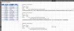
I need to first match the ID, then the VENDOR, and if the TYPE contains the words "next", then give me the largest (MAX) of the values matched. In some instances TYPE matches twice, in others one, and others none.
Ideally this would be in formula format, I can't add macros/VBA to the file.

I have tried two formulas, both with no good result, FYI, the data is formatted as a table and named DataTable.
I tried: '{=LARGE(IF(DataTable[TYPE]="*next*",INDEX(DataTable[VALUE],MATCH(1,(DataTable[ID]=G4)*(DataTable[VENDOR]=G5),0)),"not found"),1}
and I also tried: '{=LARGE(IF((DataTable[ID]=G11)*(DataTable[VENDOR]=G12)*(DataTable[TYPE]="*next*"),DataTable[VALUE],""),ROW($A$2))}
Neither of these work for me.

ID	VENDOR	TYPE	VALUE		EXAMPLE 1: LOOKUP RESULT
2​	ACME	FTL other	1.18​		ID	2
2​	ACME	Six next-day	1.25​		VENDOR	BELFRY
2​	ACME	two next day	1.25​		TYPE	*next*
2​	ACME	mixed	1.25​		VALUE	1.12​	<---correct answer from formula should be
2​	BELFRY	FTL other	1.05​
2​	BELFRY	Six next-day	1.08​
2​	BELFRY	two next day	1.12​		EXAMPLE 2: LOOKUP RESULT
2​	CROSS	FTL other	1.01​		ID	2
2​	CROSS	Six next-day	1.09​		VENDOR	ACME
2​	CROSS	two next day	1.15​		TYPE	*next*
2​	DINGO	FTL other	1.01​		VALUE	1.25​	<---correct answer from formula should be
2​	DINGO	FTL mixed	1.09​				even though both "next" matches are the same "1.25"
2​	DINGO	two next day	1.15​
					EXAMPLE 3: LOOKUP RESULT
					ID	2
					VENDOR	DINGO
					TYPE	*next*
					VALUE	1.15​	<---correct answer from formula should be
							even though there is only one "next" day match

Any help is greatly appreciated. Image attached with the scenario.

 

[DanteAmor]

Try this

Dante Amor
	A	B	C	D	E	F	G	H	I
1	ID	VENDOR	TYPE	VALUE		ID	VENDOR	TYPE	VALUE
2	2	ACME	FTL other	1.18		2	BELFRY	next	1.12
3	2	ACME	Six next-day	1.25		2	ACME	next	1.25
4	2	ACME	two next day	1.25		2	DINGO	next	1.15
5	2	ACME	mixed	1.25		2	CROSS	next	1.15
6	2	BELFRY	FTL other	1.05
7	2	BELFRY	Six next-day	1.08
8	2	BELFRY	two next day	1.12
9	2	CROSS	FTL other	1.01
10	2	CROSS	Six next-day	1.09
11	2	CROSS	two next day	1.15
12	2	DINGO	FTL other	1.01
13	2	DINGO	FTL mixed	1.09
14	2	DINGO	two next day	1.15
S2

Cell Formulas
Range	Formula
I2:I5	I2	=LOOKUP(2,1/((Table1[ID]=F2)*(Table1[VENDOR]=G2)*(SEARCH(H2,Table1[TYPE]))),Table1[VALUE])

 

[DRSteele]

Try this. depending on your version of Excel, it might need to be invoked with Ctrl+Shift+Enter.

=MAX(IFERROR(SEARCH(G6,DataTable[TYPE]),0)*(DataTable[VENDOR]=G5)*DataTable[VALUE])

 

[ripina]

Try this. depending on your version of Excel, it might need to be invoked with Ctrl+Shift+Enter.

=MAX(IFERROR(SEARCH(G6,DataTable[TYPE]),0)*(DataTable[VENDOR]=G5)*DataTable[VALUE])

Unfortunately this doesn't work, I keep receiving an error. Also is it not missing the second part for "IFERROR"?

 

[ripina]

Try this

Dante Amor
	A	B	C	D	E	F	G	H	I
1	ID	VENDOR	TYPE	VALUE		ID	VENDOR	TYPE	VALUE
2	2	ACME	FTL other	1.18		2	BELFRY	next	1.12
3	2	ACME	Six next-day	1.25		2	ACME	next	1.25
4	2	ACME	two next day	1.25		2	DINGO	next	1.15
5	2	ACME	mixed	1.25		2	CROSS	next	1.15
6	2	BELFRY	FTL other	1.05
7	2	BELFRY	Six next-day	1.08
8	2	BELFRY	two next day	1.12
9	2	CROSS	FTL other	1.01
10	2	CROSS	Six next-day	1.09
11	2	CROSS	two next day	1.15
12	2	DINGO	FTL other	1.01
13	2	DINGO	FTL mixed	1.09
14	2	DINGO	two next day	1.15
S2

Cell Formulas
Range	Formula
I2:I5	I2	=LOOKUP(2,1/((Table1[ID]=F2)*(Table1[VENDOR]=G2)*(SEARCH(H2,Table1[TYPE]))),Table1[VALUE])

This works great! I'm going to apply it to my actual data and see how it performs. Thanks for the quick reply.

 

[DRSteele]

Which version of Excel are you using?

The IFERROR function has a 0 as its condition argument.

 

[ripina]

Thanks DanteAmor, fomrula works perfectly. I'm going to research the Lookup and Search formulas to learn how they function. Would you be able to share how it works, I want to learn, not just copy and paste formulas. Thanks again.

 

[DanteAmor]

=LOOKUP(2,1/((Table1[ID]=F2)*(Table1[VENDOR]=G2)*(SEARCH(H2,Table1[TYPE]))),Table1[VALUE])

1. When the data is ordered, from least to greatest, if the LOOKUP function does not find the value, then it returns the last value of the data.

SEARCH(H2,Table1[TYPE])

2. Search, look for "next" in the column "TYPE", if it finds it, it returns a number, if it doesn't find it, it returns the error: #!Value!

3. Using the LOOKUP formula in this way "Lookup (2,1 / ...)" turns it into an array formula, that is, an array formula is a formula that can perform multiple calculations on one or more of the items in an array.

4. ((Table1[ID]=F2)*(Table1[VENDOR]=G2)*(SEARCH(H2,Table1[TYPE])) , This compares the ID with F2, the vendor with G2 and type with H2, the values that match are TRUE and those that do not match are FALSE.

5. TRUE results are converted to 1 and FALSE values are converted to 0.
6. 1/((Table1[ID]=F2)*(Table1[VENDOR]=G2)*(SEARCH(H2,Table1[TYPE]))) , 1 Divide the results TRUE or FALSE

That's
= 1/TRUE, 1/FALSE
= 1/1, 1/0
= 1/1 = 1, 1/0 = Error "#¡DIV/0!"

7. LOOKUP(2,1/((Table1[ID]=F2)*(Table1[VENDOR]=G2)*(SEARCH(H2,Table1[TYPE]))),Table1[VALUE]) Then look for the 2 in the (#¡DIV/0!, 1) vector and since it doesn't find it, then it takes the last value, in this case take the last 1.

8. Finally take the last position of the resulting vector.

I hope it helps.

 

[ripina]

Thank you very much, great explanation. I wasn't sure what the "2,1" at the beginning of the Lookup formula was doing. Very insightful, I may be able to use this for other tasks. Thanks again.

 

[DanteAmor]

I'm glad to help you. Thanks for the feedback.