Index Match Match with a loop

[MrK91]

Hello all,

New to the thread so I do apologies if this isn't sufficient.

I am trying to create VBA code for Index Match Match with a loop.

I have attached an image to help.

To detail the problem;
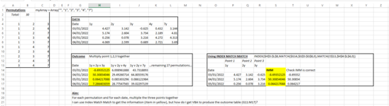
- Cells A4:C13 have permutations from myarray (1,2,3,4,7) where I want 3 numbers picked and no repeats eg 1,2,3 | 1,2,4 | etc... (macro already created).
- I have data in cells G4:L8 which gives each point (1,2,3,4,7) values based upon specific dates (3/1/22 - 6/1/22)
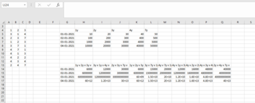
- I want to create VBA code which will use each permutation and multiply the 3 points together for each date

I can use INDEX MATCH MATCH to do this with the formula being:
=INDEX($H$5:$L$8,MATCH($O16,$G$5:$G$8,0),MATCH(P$13,$H$4:$L$4,0))*INDEX($H$5:$L$8,MATCH($O16,$G$5:$G$8,0),MATCH(Q$13,$H$4:$L$4,0))*INDEX($H$5:$L$8,MATCH($O16,$G$5:$G$8,0),MATCH(R$13,$H$4:$L$4,0))

But how do I use VBA to do this INDEX MATCH MATCH and Loop through all permutations and dates please?

Thank you very much for your help in advance and time.

 

[kvsrinivasamurthy]

AS per your data format formula In H14, then copied to full range.

=INDEX($H$5:$L$8,MATCH($G14,$G$5:$G$8,0),MATCH(OFFSET($A$4,COLUMNS($H$5:H$5)-1,0)&"y",$H$4:$L$4,0))*INDEX($H$5:$L$8,MATCH($G14,$G$5:$G$8,0),MATCH(OFFSET($B$4,COLUMNS($H$5:H$5)-1,0)&"y",$H$4:$L$4,0))*INDEX($H$5:$L$8,MATCH($G14,$G$5:$G$8,0),MATCH(OFFSET($C$4,COLUMNS($H$5:H$5)-1,0)&"y",$H$4:$L$4,0))

 

[MrK91]

AS per your data format formula In H14, then copied to full range.

=INDEX($H$5:$L$8,MATCH($G14,$G$5:$G$8,0),MATCH(OFFSET($A$4,COLUMNS($H$5:H$5)-1,0)&"y",$H$4:$L$4,0))*INDEX($H$5:$L$8,MATCH($G14,$G$5:$G$8,0),MATCH(OFFSET($B$4,COLUMNS($H$5:H$5)-1,0)&"y",$H$4:$L$4,0))*INDEX($H$5:$L$8,MATCH($G14,$G$5:$G$8,0),MATCH(OFFSET($C$4,COLUMNS($H$5:H$5)-1,0)&"y",$H$4:$L$4,0))

Thank you for your help Kvsrinivasamurthy,
1. May I ask how one would loop through the permutations in cells A4:C13 to then calculate the values for each (ie 3 times)
2. I have used hard formulas below and items such as Selection.FillDown is there a better way of doing this?


My code currently looks as follows;

Sub Calc()

'Formula for Index Match Match (IMM)and drag down the formula
Range("G24").FormulaR1C1 = _
"=INDEX(R5C8:R8C12,MATCH(R[-19]C7,R5C7:R8C7,0),MATCH(R4C[-6]&""y"",R4C8:R4C12,0))*INDEX(R5C8:R8C12,MATCH(R[-19]C7,R5C7:R8C7,0),MATCH(R4C[-5]&""y"",R4C8:R4C12,0))*INDEX(R5C8:R8C12,MATCH(R[-19]C7,R5C7:R8C7,0),MATCH(R4C[-4]&""y"",R4C8:R4C12,0))"
Range("G24:G27").Select
Selection.FillDown

'Formula to copy and paste date
Range("F23").Select
ActiveCell.FormulaR1C1 = "=R[-19]C[1]"
Range("F23:F27").Select
Selection.FillDown

'Formula to name
Range("G23").Select
ActiveCell.FormulaR1C1 = _
"=R[-19]C[-6]&""y v ""&R[-19]C[-5]&""y v ""&R[-19]C[-4]&""y """
Range("G24").Select
Sheet1.Range("F24", "F50000").NumberFormat = "dd/mm/yyyy"

End Sub

 

[kvsrinivasamurthy]

For the given data I have given code . Adjust ranges as required. G13:Q17 is the result of macro.

Sub Macro1()
Dim T  As Integer
Range("G5:G8").Copy Range("G14")  'copy dates to G14 and down
Range("H14:Q17").Formula = "=INDEX($H$5:$L$8,MATCH($G14,$G$5:$G$8,0),MATCH(OFFSET($A$4,COLUMNS($H$5:H$5)-1,0)&""y"",$H$4:$L$4,0))*INDEX($H$5:$L$8,MATCH($G14,$G$5:$G$8,0),MATCH(OFFSET($B$4,COLUMNS($H$5:H$5)-1,0)&""y"",$H$4:$L$4,0))*INDEX($H$5:$L$8,MATCH($G14,$G$5:$G$8,0),MATCH(OFFSET($C$4,COLUMNS($H$5:H$5)-1,0)&""y"",$H$4:$L$4,0))"
For T = 4 To 13    'Row numbers for A4:C13 range
Range("H13").Offset(0, T - 4) = Range("A" & T) & "y v " & Range("B" & T) & "y v " & Range("C" & T) & "y"  'Headings from H13 to right
Next T
Range("H14:Q14").EntireColumn.AutoFit
End Sub

 

[kvsrinivasamurthy]

I have modified the code.
Starting cell of result is G14. You are required to change only G14 and H14 depending on your requirement.

Sub Macro2()
Dim T  As Integer
Dim LR As Long
Range("G5:G8").Copy Range("G14")  'copy dates to G14 and down
LR = Range("G14").End(xlDown).Row  ' last row number
Range("H14:Q" & LR).Formula = "=INDEX($H$5:$L$8,MATCH($G14,$G$5:$G$8,0),MATCH(OFFSET($A$4,COLUMNS($H$5:H$5)-1,0)&""y"",$H$4:$L$4,0))*INDEX($H$5:$L$8,MATCH($G14,$G$5:$G$8,0),MATCH(OFFSET($B$4,COLUMNS($H$5:H$5)-1,0)&""y"",$H$4:$L$4,0))*INDEX($H$5:$L$8,MATCH($G14,$G$5:$G$8,0),MATCH(OFFSET($C$4,COLUMNS($H$5:H$5)-1,0)&""y"",$H$4:$L$4,0))"
For T = 4 To 13    'Row numbers for A4:C13 range
Range("G14").Offset(-1, T - 3) = Range("A" & T) & "y v " & Range("B" & T) & "y v " & Range("C" & T) & "y"  'Headings from H13 to right
Next T
Range("G14:Q14").EntireColumn.AutoFit
End Sub

 

[MrK91]

I have modified the code.
Starting cell of result is G14. You are required to change only G14 and H14 depending on your requirement.

Sub Macro2()
Dim T  As Integer
Dim LR As Long
Range("G5:G8").Copy Range("G14")  'copy dates to G14 and down
LR = Range("G14").End(xlDown).Row  ' last row number
Range("H14:Q" & LR).Formula = "=INDEX($H$5:$L$8,MATCH($G14,$G$5:$G$8,0),MATCH(OFFSET($A$4,COLUMNS($H$5:H$5)-1,0)&""y"",$H$4:$L$4,0))*INDEX($H$5:$L$8,MATCH($G14,$G$5:$G$8,0),MATCH(OFFSET($B$4,COLUMNS($H$5:H$5)-1,0)&""y"",$H$4:$L$4,0))*INDEX($H$5:$L$8,MATCH($G14,$G$5:$G$8,0),MATCH(OFFSET($C$4,COLUMNS($H$5:H$5)-1,0)&""y"",$H$4:$L$4,0))"
For T = 4 To 13    'Row numbers for A4:C13 range
Range("G14").Offset(-1, T - 3) = Range("A" & T) & "y v " & Range("B" & T) & "y v " & Range("C" & T) & "y"  'Headings from H13 to right
Next T
Range("G14:Q14").EntireColumn.AutoFit
End Sub

Thank you very much for your help and time. This is exactly what I was after and works perfectly.

I have added in some dynamic range names to replace the likes of H5:L8 etc.

Thank you again for your help

 

[kvsrinivasamurthy]

Welcome