Index/Match/Maxifs Question

[Marter]

Hello,

I'll explain what I'm trying to do then tell you what I'm currently doing that isn't working as I want it to.

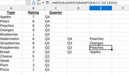
What I'm trying to do. I want a formula to return text from Column A based on the highest number in Column B, but only in cells that match Column C.

I've attached a photo.

Essentially I only want the highest result for each quarter.

In the example I listed above, this works for Q4 and Q3 but not for Q2 and Q1. The photo has the formula for Q2 but I'll post it here as well:

=INDEX(A:A,MATCH(MAXIFS(B:B,C:C,"Q2"),B:B,0))

The formulas are all the same, just the "Q#" is changed.

What it's doing is searching based on the criteria but then giving me the first result with criteria ignored. So for Q2 it sees that "Strawberries" with an 8 is the highest, but then it spits out "Peaches" as that's the first 8 in the column, even though I told it only ones that match Q2.

Please let me know what I'm doing wrong and what I can do to achieve what I need.

Thanks!

 

[Marcelo Branco]

Try...

Pasta1
	A	B	C	D	E
1	Type	Rating	Quarter
2	Apples	7	Q4
3	Pears	6	Q4
4	Peaches	8	Q4
5	Oranges	9	Q3
6	Blueberries	1	Q3
7	Watermellon	6	Q3	Q4	Peaches
8	Strawberries	8	Q2	Q3	Oranges
9	Raspberries	4	Q2	Q2	Strawberries
10	Bread	3	Q2	Q1	Steak
11	Cheese	5	Q1
12	Steak	7	Q1
13	Plum	3	Q1
14	Pizza	1	Q1
Plan4

Cell Formulas
Range	Formula
E7:E10	E7	=INDEX(A$2:A$14,AGGREGATE(15,6,(ROW(A$2:A$14)-ROW(A$2)+1)/((C$2:C$14=D7)*(B$2:B$14=AGGREGATE(14,6,B$2:B$14/(C$2:C$14=D7),1))),1))

Hope this helps

M.

 

[Marter]

That does indeed work. I do not understand it but it seems to work! Thanks!

 

[Marter]

Try...


M.

Actually, one more question!

How would I reverse this to look for lowest instead of highest?

 

[Marcelo Branco]

How would I reverse this to look for lowest instead of highest?

Try

Pasta1
	A	B	C	D	E	F	G
1	Type	Rating	Quarter
2	Apples	7	Q4
3	Pears	6	Q4
4	Peaches	8	Q4
5	Oranges	9	Q3
6	Blueberries	1	Q3		Highest		Lowest
7	Watermellon	6	Q3	Q4	Peaches		Pears
8	Strawberries	8	Q2	Q3	Oranges		Blueberries
9	Raspberries	4	Q2	Q2	Strawberries		Bread
10	Bread	3	Q2	Q1	Steak		Pizza
11	Cheese	5	Q1
12	Steak	7	Q1
13	Plum	3	Q1
14	Pizza	1	Q1
Plan4

Cell Formulas
Range	Formula
E7:E10	E7	=INDEX(A$2:A$14,AGGREGATE(15,6,(ROW(A$2:A$14)-ROW(A$2)+1)/((C$2:C$14=D7)*(B$2:B$14=AGGREGATE(14,6,B$2:B$14/(C$2:C$14=D7),1))),1))
G7:G10	G7	=INDEX(A$2:A$14,AGGREGATE(15,6,(ROW(A$2:A$14)-ROW(A$2)+1)/((C$2:C$14=D7)*(B$2:B$14=AGGREGATE(15,6,B$2:B$14/(C$2:C$14=D7),1))),1))

Note that the only difference between the formulas is in the second AGGREGATE function: to get the Largest I used 14 as the first parameter; to get the Smallest one, I used 15 as the first parameter.

Take a look at Help about the AGGREGATE function

AGGREGATE function - Microsoft Support

The AGGREGATE function can apply different aggregate functions to a list or database with the option to ignore hidden rows and error values.

support.microsoft.com

M.

 

[Marter]

Note that the only difference between the formulas is in the second AGGREGATE function: to get the Largest I used 14 as the first parameter; to get the Smallest one, I used 15 as the first parameter.

Take a look at Help about the AGGREGATE function

AGGREGATE function - Microsoft Support

The AGGREGATE function can apply different aggregate functions to a list or database with the option to ignore hidden rows and error values.

support.microsoft.com

M.

I had tried that because I figured it was something like that and it kind of worked ... but it counts blank cells as the lowest. Is there a way it can only target filled cells?

 

[Marcelo Branco]

I had tried that because I figured it was something like that and it kind of worked ... but it counts blank cells as the lowest. Is there a way it can only target filled cells?

Could you provide an example with blank cells you're getting wrong results?

M

 

[Marter]

Could you provide an example with blank cells you're getting wrong results?

M

Sure thing! I tried using the Mini-sheet but it wouldn't work, sorry. Have to do with pictures and written formulas.

In the picture, all of the blanks have taken precedence over the actual lowest numbers. The formulas are:

=INDEX(A$2:A$14,AGGREGATE(15,6,(ROW(A$2:A$14)-ROW(A$2)+1)/((C$2:C$14=D7)*(B$2:B$14=AGGREGATE(15,6,B$2:B$14/(C$2:C$14=D7),1))),1))

=INDEX(A$2:A$14,AGGREGATE(15,6,(ROW(A$2:A$14)-ROW(A$2)+1)/((C$2:C$14=D8)*(B$2:B$14=AGGREGATE(15,6,B$2:B$14/(C$2:C$14=D8),1))),1))

=INDEX(A$2:A$14,AGGREGATE(15,6,(ROW(A$2:A$14)-ROW(A$2)+1)/((C$2:C$14=D9)*(B$2:B$14=AGGREGATE(15,6,B$2:B$14/(C$2:C$14=D9),1))),1))

=INDEX(A$2:A$14,AGGREGATE(15,6,(ROW(A$2:A$14)-ROW(A$2)+1)/((C$2:C$14=D10)*(B$2:B$14=AGGREGATE(15,6,B$2:B$14/(C$2:C$14=D10),1))),1))

So like for Q4 if I put in a 7 for Apples it correctly adjust so that Peaches is the lowest. But when it's blank, that's what it uses.

Hope that makes sense!

 

[Marcelo Branco]

Try

Pasta1
	A	B	C	D	E	F	G
1	Type	Rating	Quarter
2	Apples		Q4
3	Pears	6	Q4
4	Peaches	8	Q4
5	Oranges	9	Q3
6	Blueberries		Q3		Highest		Lowest
7	Watermellon	6	Q3	Q4	Peaches		Pears
8	Strawberries	8	Q2	Q3	Oranges		Watermellon
9	Raspberries		Q2	Q2	Strawberries		Bread
10	Bread	3	Q2	Q1	Steak		Pizza
11	Cheese	5	Q1
12	Steak	7	Q1
13	Plum		Q1
14	Pizza	1	Q1
15
Plan2

Cell Formulas
Range	Formula
E7:E10	E7	=INDEX(A$2:A$14,AGGREGATE(15,6,(ROW(A$2:A$14)-ROW(A$2)+1)/((C$2:C$14=D7)*(B$2:B$14=AGGREGATE(14,6,B$2:B$14/(C$2:C$14=D7),1))),1))
G7:G10	G7	=INDEX(A$2:A$14,AGGREGATE(15,6,(ROW(A$2:A$14)-ROW(A$2)+1)/((C$2:C$14=D7)*(B$2:B$14=AGGREGATE(15,6,B$2:B$14/(ISNUMBER(B$2:B$14)*(C$2:C$14=D7)),1))),1))

M.

 

[Marter]

Perfect! Thank you so much for your help!